Table of Contents
3.5.2. Zoom out last level option
3.5.3. Zoom out all levels options
4.3.2. Advance Function Editor
4.9.3. List of formulas to evaluate
4.9.7. Editing the list of formulas
5.2.3. Cumulative sum – cumsum
5.2.12. Phase Difference – phasediff
5.2.13. Phase shift – phaseshift
5.2.21. Window_Average_Value – wavg
5.2.22. Window_Maximum_Value – wmax
5.2.23. Window_Minimum_Value – wmin
5.2.24. Window_RMS_Value – wrms
5.2.25. Window_Sum_Value – wsum
5.3.1. 3 Phase Power – power3ph
5.3.3. Clearing time – clearingtime
5.3.7. Peak of Envelop – envpeak
5.3.8. Envelope Phase–Phase – envpp
5.3.9. Product of time step and square of the input – I2T
5.3.10. Instantaneous_Power – Power
5.3.13. Maximum_Finite_Value – maxf
5.3.14. Minimum_Finite_Value – minf
5.3.16. Operation Time – optime
5.3.20. Threshold_Time – thresholdtime
5.4.1. Cumulative_Probability – cumprob
5.4.2. Gaussian_Distribution – gauss
5.4.3. Mean Deviation – meandev
5.4.5. Standard deviation – stddev
5.4.6. Statistical_Frequency – statfreq
5.5.1. Fast Fourier Transform – fft
5.5.2. Fundamental Frequency – ffreq
5.5.3. Fundamental Frequency Signal – ffreqs
5.5.7. Sequence impedance – zseq
5.5.8. Symmetrical_Component_Module – syhmod
5.5.9. Symmetrical_Component_Phase – sypha
5.5.10. Total_Harmonic_Distortion – thd
5.6.1. Linear_Interpolation – interpl
5.7.1. Type of windows for the following functions:
5.7.2. Cross_Spectral_Density – crospec
5.7.3. Frequency_Response – repfreq
5.7.4. Spectral_Density – densp
5.8.1. Overshoot time – sidseuil
5.8.2. Fundamental Frequency – sifreq
5.8.3. Absolute Maximum – simax1
5.8.4. Absolute Maximum – simax2
5.8.7. Harmonic Maximum – simxhart
5.8.8. Integral maximum – simxsom1
5.8.9. Integral maximum – simxsom2
5.8.10. Dynamic Response – sidyn2
5.8.11. Absolute harmonic maximum – simxsymt
5.8.12. Power and impedance – sipz
5.8.13. Overshoot Statistics – siseuil
5.8.14. Symmetric components – sisym3
5.8.15. Envelope Overshoot– sitenv
5.8.16. Operating time – Sitop
5.8.17. Relative operating time – sitopref
5.8.18. Threshold time – sitseuil
SCOPEVIEW is a mathematical and graphical data acquisition and signal processing software. It is used to simultaneously view and process data from many sources, such as:
HYPERSIM®;
EMTP-RV;
EMTP-V3 .pl4 files;
MATLAB and;
COMTRADE.
The results are displayed graphically for further analysis and processing.
ScopeView:
Runs under Unix®;
Runs under Linux® RedHat 7.2 / 7.3 with Linux 2.4 kernel;
Runs under Linux® Enterprise WS4 with Linux 2.6 kernel:
Runs under Windows®;
Supports off-line and real-time simulations.
Here are the main features of the software:
Simultaneously view and process data from many sources (multi source and multi domain);
Execute a variety of mathematical functions on signals (e.g. spectral density, frequency re-sponse, coherence, etc.);
Offer an interpreter for mathematical formulas that handle signals and scalars;
Execute many types of graphic processing on signals (e.g. zoom, superimposition, versus, tracking cursor, interactive displacement of graphs, etc.);
Save signal processing and editing information in a model acquisition file for later use;
Allow exporting signals acquired in different formats (e.g. MATLAB, ASCII, PDF, POST-SCRIPT)
ScopeView may be used in either English or French.
In Microsoft Windows:
From the Windows control Panel, click on the Regional Settings;
In the General Options, select English (Canada) or French (Canada);
Launch ScopeView.
To change ScopeView language, if it’s already running, shut down ScopeView, change the language setting then start ScopeView again.
This is a quick tutorial to use ScopeView and to be used as an example.
Launch HYPERSIM®[1] and load the CIGRE_3 example file.
Start the simulation.
Load sensors using the saved signals file.
Launch ScopeView.
Click on the Data Source button in the Signals Window of ScopeView. Then select HYP tab and Load.
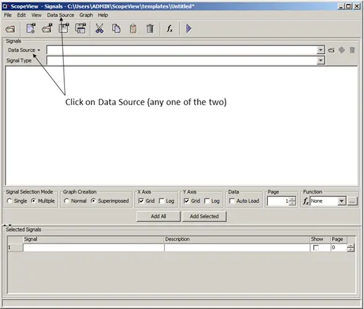
Figure 1: ScopeView Signal Form Window
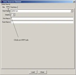
Figure 2: Data Sources Chooser
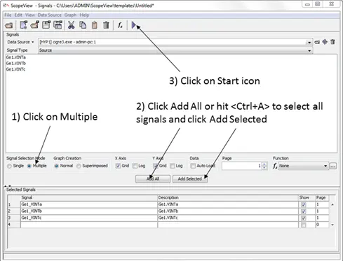
Figure 3: Signals displayed
Using the mouse left click, select signals from the top part of the signal window. The chosen signals move automatically to the Selected Signals table at the bottom of the window.
Select all signals by clicking on Add All or use <Ctrl+A> keys to select all the signals at once then click on the Add Selected button.
Finally, click on the Start icon.
Results are displayed in the ScopeView Graphic.
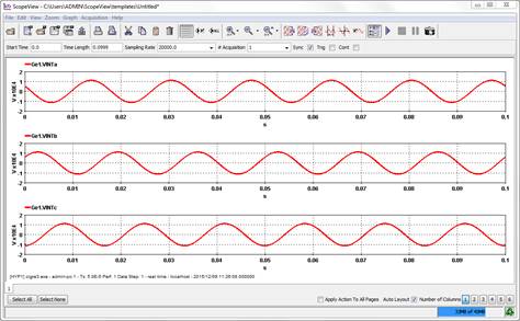
Figure 4: Results displayed in the Graphic Page
When ScopeView opens, the Signals form and the Main window are present on the screen. The ScopeView Signals form shows on top of the main window in order to first choose a source of signals and a template to be displayed by the Main window.
The Main window is described in this Chapter and the Signals form features are presented in Chapter 4.
This section describes the major elements displayed in the main window of ScopeView. For a clearer understanding, it is subdivided in different areas, which are described in this chapter. These areas are the following:
Control buttons area.
Graphic page area.
Edit graphs area.
Information area.
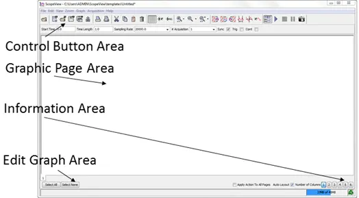
Figure 5: Main Window Area
The two following figures give a brief description of each control button. The same shows a description that will appear when you leave your mouse cursor on the chosen button.
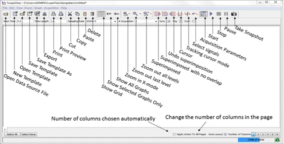
Figure 6: Icon related function
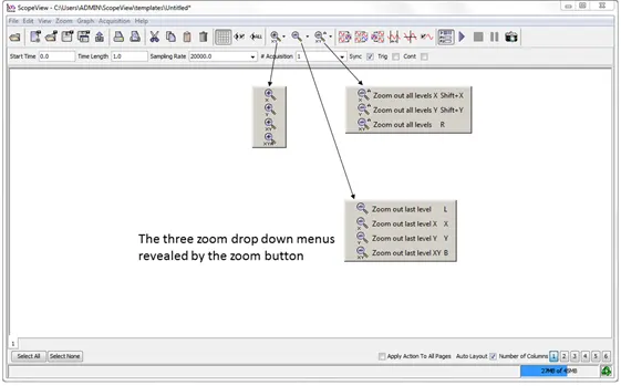
Figure 7: Zoom options
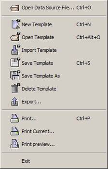
Figure 8: File menu
3.2.1.1. Open Data Source File...
Displays the window below. Select a file that was previously generated or select HYP for connecting to a HYPERSIM® model, TestView to connect to a TestView model. Clicking Load will load the data source of interest.
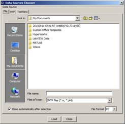
Figure 9: Data sources chooser window File and HYP tabs
3.2.1.2. New Template
This item from the menu clears the graphic page area to let you create your own new template.
3.2.1.3. Open Template
Allows opening template used with another simulation session. Template files have.xml or.mod extension. The name of the template file will then appear at the top of the main window.

Figure 10: Open Template Window
3.2.1.4. Save Template
Allows saving a study set-up in a file for future use as a template or to help in setting up a new study in your current directory. The template is saved under ScopeView\templates\...
3.2.1.5. Save Template As...
Allows to save a study set-up in a file for future use as a template or to help in setting up a new study in the directory of your choice.
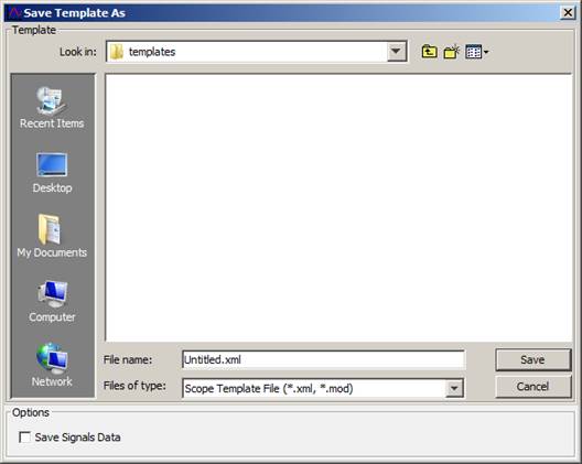
Figure 11: Save Template As window
3.2.1.6. Delete Template
To erase a template from your work station
3.2.1.7. Export...
Used to transfer a result file in a different format to be used with simulation software or in a convenient format for visualization or printing purposes. Available formats are:
Comtrade (*.cfg)
Encapsulated Post Script (EPS) (*.eps);
Joint Photographic Expert Group (*.jpg)
MATLAB Binary (*.mat);
Portable Document Format (PDF) (*.pdf);
Portable Network Graphic (*.webp);
Post Script (PS) (*.ps);
Text (tab separator) (*.txt).
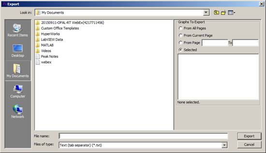
Figure 12: Export Action Window
3.2.1.8. Print...
Print the actual window (results) displayed on screen. Allows selecting one of the printers installed on your workstation.
3.2.1.9. Print preview...
Displays the actual graphical page area (results) before printing is released.
3.2.1.10. Exit
Quits and closes ScopeView.

Figure 13: Edit menu
3.2.2.1. Cut
Select a graph from the main window and click on this function to remove the graph from the graphic page area and put it on the clipboard.
3.2.2.2. Copy
Select the graph you want and click on this function to copy the graph on the clipboard. The selected graph remains on the graphic page area.
3.2.2.3. Paste
This function displays the content of the clipboard on the actual graphic page area.
3.2.2.4. Paste on a new page
A variant from the Paste option. This function will create a new page and displays the content of the clipboard.
3.2.2.5. Delete
Remove definitely the selected graph from graphic page area displayed.
3.2.2.6. Select All
Select all the graphs displayed on the graphic page area.
Another way to select all graphs is, move the cursor in the graphic page area then press the <CTRL> and <a> keys.
3.2.2.7. Select None
Deselect all the graphs selected before.
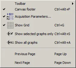
Figure 14: View menu
3.2.3.1. Toolbar
Allows user to show or hide the different menus from the Toolbar.
3.2.3.2. Canvas Footer
Allows showing or hiding the Edit Graph buttons at the lower left hand side of the ScopeView window.
3.2.3.3. Acquisition parameters...
Allows selecting the starting time, sampling time length (duration) and, number of acquisitions to execute.
Synchronization (when ticked) specifies if a synchronization signal should be used during data acquisition[2].
3.2.3.4. Show Grid
Displays grid on all graphs on the graphic page area.
3.2.3.5. Show selected graphs only
Select the graph(s) you want to display and click on this option.
If you select, for example, only one graph, the later will occupy the complete area of the graphic page area.
Unselected graphs are hidden not deleted.
3.2.3.6. Show all graphs
Displays all the graphs including the ones that were hidden before.
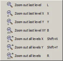
Figure 15: Zoom Menu
The zoom options from the menu or the control buttons at the top of the main window allow viewing parts of graphs with a greater resolution in order to focus on selected parts of graphs.
The following types of zoom are available:
X;
Y;
XY;
X Y Auto;
Moreover, ScopeView remembers the zooms made to revert to a previous state or an original state.
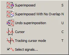
Figure 16: Graph menu
3.2.5.1. Superimposed
ScopeView will display two or more traces in the same graph (depending how many signals you have selected).
3.2.5.2. Undo Superimposed
ScopeView will display one signal per graph.
3.2.5.3. Cursor
ScopeView will display a Region cursor and a corresponding table. This type of cursor selects an area of interest of a graph and displays the coordinates and other information as per the table below.
To activate this feature, select the Cursor item; click your mouse to the beginning of the area you want then at the other end of the same area.
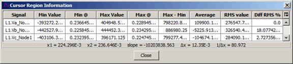
Figure 17: Region cursor table
3.2.5.4. Tracking Cursor Mode
Change the default cursor to a cross-hair cursor. The tracking cursor follows the graph curve and displays axis values at the lower left hand side of the graph.
To activate the cross-hair cursor function, first select the graph(s) of interest.
To select many graphs, press and hold the <CTRL> key then click on the graphs you want to select.
To select all the graphs, click on the Select All button at the lower left corner of the graphic page area.
Once the data acquisition is executed, the software displays the results graphically. It is possible to process and analyse the acquired signals. This section covers the part after the acquisition, which is usually referred to as post processing.
This section explains the different methods used to access post-processing functions. Since many of these functions require the selection of one or many graphs, the method used to select graphs is also described.
Most of the post processing functions offered by ScopeView can be selected from the tool bar or the background menu of the graphic page area.
Most graphic actions can be executed on one or many graphs simultaneously. The software uses a general procedure to select graphs of interest.

Figure 18: Graph Selection
3.3.1.1. To select graphs of interest:
Hold down the <CTRL> key and click on each graph of interest. A frame is displayed around the graph.
Deselect a graph by holding down the <CTRL> key and clicking on the graph again. The frame disappears.
3.3.1.2. To select all the graphs simultaneously:
Use the Edit Graph buttons at the left bottom corner of the window.
3.3.1.3. To deselect the graphs:
Use the Edit Graph buttons at the left bottom corner of the window. Or from Edit menu, choose Select None (<Ctrl+Alt+N>) item.
3.3.1.4. Editing
This section details the methods available to edit each graphic page created during an acquisition. The following topics are covered:
Selecting the Graphic page to display;
Graph layout;
Changing the appearance of graphs;
Editing form;
Adding specific notes;
Saving the editing information. (ScopeView saves the editing information in the template files).
3.3.1.5. Selecting the Graphic page to Display
The Page selection tab at the bottom of the Graphic page enables you to navigate between the different graphic pages created during an acquisition.
To change the graphic page to be displayed, click on the desired page tab at the bottom in the main window.
3.3.1.6. Graph Layout
Changing the Number of Columns. You can change the number of columns of the current page using the Number of columns item at the bottom of the graphic page.
For ease of use, the software allows a maximum of six columns and each column can consist of six graphs. ScopeView will deny or change without a warning message any selection over¬riding this limit.
To change the number of columns in the current page: Click on the number of columns you want in the Number of Columns buttons at the bottom of the main window.
3.3.1.7. Auto layout
The Auto layout button tells ScopeView if it should or not arrange graphs automatically when changing the number of columns in a graphic page. In automatic mode, ScopeView attempts to place an identical number of graphs in each column.
3.3.1.8. Moving Graphs Manually
To allow for the maximum of freedom in editing graphs, ScopeView offers the possibility of moving a graph interactively to another location in the same column, in a different column or even to another graphic page.
3.3.1.9. Moving Many Graphs to Another Page:
Select the graphs to be moved;
From the background menu, select Copy;
Then, select Paste on a new page.
If you select a graph then select Paste on a new page without selecting Copy, ScopeView will create a new page (after the last one) and will move the graph. Or, select the destination page from the page tabs and select Paste. ScopeView then moves the graph to the last column on the destination page.
3.3.1.10. To move a graph to another location on the same page:
Select the graph of interest;
Move the cursor in the top banner and a small hand will appear;
Press and hold the mouse left button to grab and move the graph to the desired position in the page. Release the button.
To display the background menu of the Graphic page, position the cursor on the graphic page;
Click the mouse right button.

Figure 19: Background Menu
The left (or top) series of icons have been described in Section Edit Menu and are standard MS Windows icons and functions.
Grid item allows showing or hiding the grid in the selected graph.
To add a grid to the graph, select the graph(s); from the background menu select Grid then Show from the sub-menu.
To hide a grid from a graph, select the graph(s); from the background menu select Grid then Hide from the sub-menu
X and Y type axis item allows the user to select either Linear or Logarithmic type of graph.
Window Properties opens an info form (see Figure 3-15) that displays the software identification; the software icon used on the graphic area page and the computer user ID.
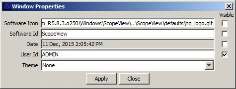
Figure 20: Window Properties
Page Properties opens the following form:
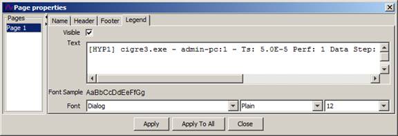
Figure 21: Page Properties
ScopeView allows you to customize editing of each page used for acquisition. You can change or add information relating to each page and also control the display of such information.
Header tab. Used to display a header title on the top of the page.
Footer tab. Used to display a footer title at the bottom of the page.
Graph Properties allows the user to change many aspects of the selected graph. Not selected graph can be modified from the list displayed at the left of the form.
Type tab displays the ordinary line traced on the graph page;
X and Y axis tabs allows to change the selected graph title, text and unit factor;
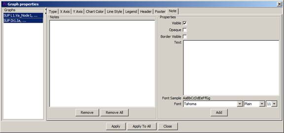
Figure 22: X and Y axis tabs
Label can be either scientific or engineer;
The scale minimum/maximum can be set to the user needs; same for the tick marks spacing and precision and;
Grid can be changed from linear to logarithmic.
Chart colour tab allows the user to change the colour of
(i) Chart
(ii) Chart Area
(iii) Plot Area
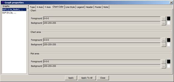
Figure 23: Chart Colour Tab
Chart
Foreground: Graph title.
Background: Banner above graph.
Chart area
Foreground: X and Y axis units’ characters.
Background: Graph background (behind the plot area).
Plot area
Foreground: X and Y axis lines.
Background: Graph drawing area inside X and Y axis.
Line style tab displays this mode of the graph properties form.
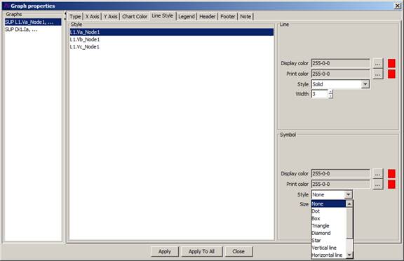
Figure 24: Line Style Tab
The plotted line colour can be changed as per the user needs;
It is also possible to use symbols on the plotted line with user-defined size and colour.
Legend tab allows to display or not the title show at the top of the chart.
Header and Footer tabs are used to add text or comments in the Header/Footer areas.
A note can be added to the plotted area of the selected chart from this mode of the Graph properties form.
To add a note to a graph, select the Note tab from the Graph Properties window, enter the desired note in the text field then click the Add button to move the text in the Notes field.
Select the note you want to see in the graph from the Notes field and click Apply.
You can drag and drop the note anywhere on the graph.
To erase a note, select the Remove or the Remove all button to erase the note. Click Apply.
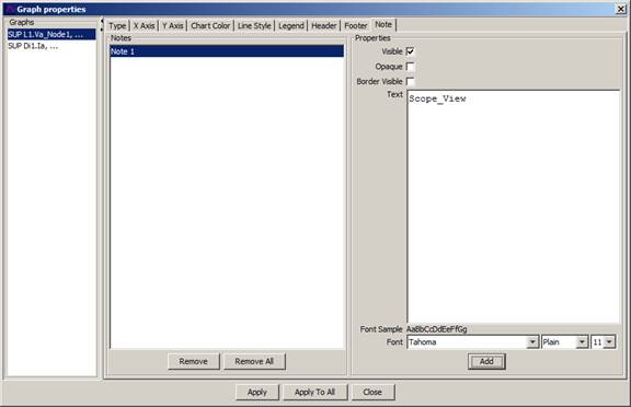
Figure 25: Note Tab
Select the format you want to store information on the clipboard (from the Copy command/ icon) to be printed, pasted or exported. To copy and paste in Word, use Bitmap, to export use Encapsulated PostScript.
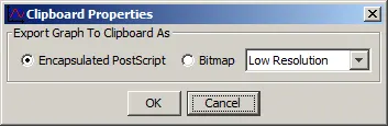
Figure 26: Clipboard Properties
To accelerate handling, the most common graphic page functions can also be accessed directly through the buttons at the top of the graphic page. For example, one of the buttons allows you to zoom in quickly on the selected graphs.
The Zoom options from the tool bar menu or from the accelerator buttons allow viewing parts of graphs with a greater resolution in order to focus on selected parts of the graphs.
Moreover, ScopeView stores the zooms made to revert to a previous state or an original state.
![]()
Figure 27: Zoom In Options
To execute an X zoom, click on the graph(s) of interest;
Then click the button at the top of the graphic page.
Position the mouse cursor at the left of the region of interest. Hold down the left button then drag the mouse to the right to sweep the region of interest and finally, release the button.
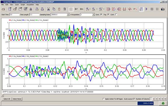
Figure 28: Before and After Zooming X Axis
There is almost no limit to the number of horizontal zooms that can be applied to a given curve. The only limit is that at least two points should always be displayed.
There are two ways to cancel the effect of zooms in: last or all levels.
3.5.2. Zoom out last level option
The last level option of the tool bar allows reverting one-step to the previous zoom. ScopeView cancels only the effect of the last step.
To execute a last level zoom out, click on the graph(s) of interest then click the button in the tool bar.
The selected graph(s) reverts to the last level in X-axis automatically;
The same action can be performed in Y-axis or in XY axis together as per the icon selected respectively.
3.5.3. Zoom out all levels options
The All levels option allows you to revert to the initial display state. ScopeView then cancels the effect of all the previous zooms.
To execute a global zoom out, click on the graph(s) of interest then click the button in the tool bar.
The selected graph(s) reverts to the original level in X-axis automatically;
The same action can be performed in Y-axis or in XY axis together as per the icon selected.
ScopeView enables you to execute many graphic actions on one or many graphs in the current page. These actions are intended to facilitate analyzing the results. The Advance Graphic Actions are:
Superimposition;
Undo superimposition`;
Cursor;
Tracking cursor;
Select Signals;
Plot signals.
In order to provide a simple way of comparing curves, you can superimpose them on the same graph. Moreover, ScopeView saves all the super impositions made to revert to each of the previous acquisitions.
To execute a Superimposition, click on the graph(s) of interest then click the button in the tool bar. The selected graphs will superimpose automatically.
Superimposition is also available in the ScopeView – Signals window.
If the graphs of interest do not have the same X display range, ScopeView then uses the union of these ranges, in other words the minimum lower delimiter and the upper maximum delimiter of all the graphs to superpose.
A different colour and type of trace is used to set apart each of the superimposed curves. A legend at the top of the graph identifies each curve.
When executing a superimposition, the selected graphs are hidden and the resulting graph is displayed at the position of the first selected graph.
The undo option of the Graph menu allows you to cancel the superimposition and return to the initial configuration.
To revert from a superimposition of graphs, select the graph of interest then click the button in the tool bar. The selected graph will revert to their original state automatically.
The “revert” superimposition is also available in the ScopeView – Signals window.
With the tracking cursor, ScopeView gives you the possibility of measuring signals displayed on the graphic page.
To switch to the tracking mode, click the cross-hair cursor icon in the tool bar. ScopeView displays the Tracking cursor on all graphs selected on the graphic page
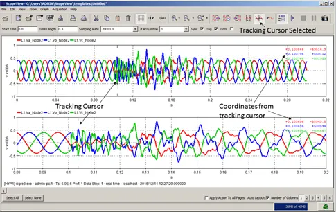
Figure 29: Tracking Cursor
To switch off the tracking mode click the cross-hair cursor icon again. It has a toggle action.
It also displays, on the status line, the coordinates of the current point of each curve (simultaneously above each graph). ScopeView updates instantaneously the coordinates when the cursor moves.
In tracking mode, you can:
Move the cursor by moving the mouse laterally. A lateral displacement brings about the automatic positioning of the horizontal line on the current point. The intersection of the vertical line with the horizontal line indicates the position of the point whose coordinates are displayed on the status line.
Use the LEFT or RIGHT arrow keys to move from one point to another on the curve.
Use the UP or DOWN arrow keys or the space bar to move the cursor from one curve to another (superimposition).
The Cursor, or the region cursor, allows the user to delimit a region of interest on the graph and display a pop-up result window. This function is very useful to compare a wider range of information, particularly in superimposed graphs, than with the tracking cursor. The tracking cursor displays results in an information window.
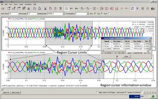
Figure 30: Region Cursor
It is possible to transfer a result file in a different format to be used with simulation software or in a convenient format for visualization or printing purposes. Available formats are:
Comtrade (*.cfg)
Encapsulated Post Script (EPS) (*.eps);
Joint Photographic Expert Group (*.jpg)
MATLAB Binary (*.mat);
Portable Document Format (PDF) (*.pdf);
Portable Network Graphic (*.webp);
Post Script (PS) (*.ps);
Text (tab separator) (*.txt).
To export a result file, click on the Export button at the top of the window
Type in the file name
Then select the file format;
Click the Export button.
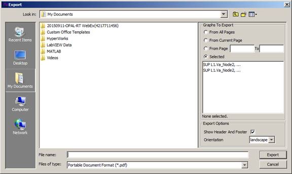
Figure 31: Exporting Results Window
The Print button in the main window is used to print the content of the graphic page with a PostScript laser printer, or to a PostScript format file.
It is possible to change the printer or the print orientation by modifying the items on the Print Options form.
To access the Print Options form, click the print button or click the print option from the File menu
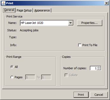
Figure 32: Print Options Window
Select the desired options.
In accordance with the printer installed on your system, select the desired options from the General, Page set-up and Appearance tabs.
Each printer and system have different options like colour output, A4 or A3 paper size etc. It is up to the user to set his printer. ScopeView on Personal Computer (PC) uses the MS Windows® drivers.
It is necessary to configure a series of items before starting data acquisition. For example, you must select the signals to acquire, the corresponding mathematical operations to perform and to specify the number of acquisition. This is the preparation phase of the acquisition and this chapter describes the steps involved.
In the Signals Form below, four areas are accessible:
The command buttons area;
The available signals area;
Signal processing;
The selected signals area
Figure 33: Signal Form Window
In the following Figure, the File and Edit menus have the same functions as already described.
Figure 34: ScopeView - Signals form
Figure 35: View Menu
Allows user to show or hide the different menus from the Toolbar.
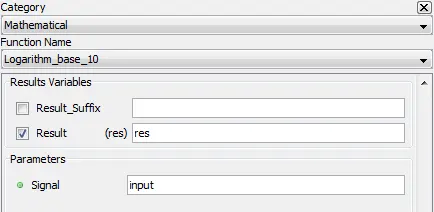
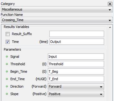
4.3.2. Advance Function Editor
Allows user to display the advanced mathematical functions in editor mode. Detailed instruction on this mode is given later.
Figure 36: Signals form in Advance Function Editor mode
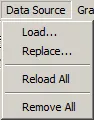
Figure 37: Data source menu
Displays the Data Sources Chooser window and allows the user to load a particular plot file or signals from Hypersim® sensors.
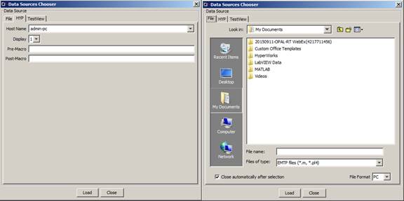
Figure 38: Data sources chooser window
Displays the Data Sources Chooser window and allows the user to replace (delete the previous if any) and load a new file.
The Data Sources Chooser window displays a Replace button instead of the Load button.
Reload the plot file already loaded when new sensors had been added in your HYPERSIM® simulation as per example.
Remove all the data sources already loaded.
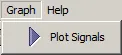
Figure 39: Graph menu
Traces the graphs from the selected signals displayed in the selected signals area of the Signals window.
This menu item is the same command as the Plot icon on the tool bar or the Start button at the top of the window.
The first group of buttons at the left of the window are the usual functions from MS Window®.
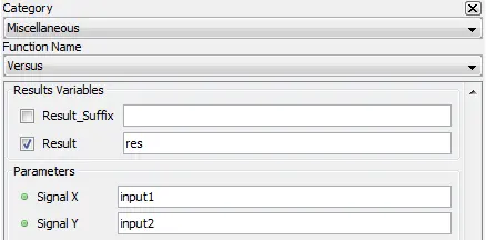
The button gives you access to the mathematical functions. (The access is duplicated at the far right middle of the window).
The Start button tells ScopeView to trace the selected signals in the graphic page area.
This area gives a detailed list of the available signals from the selected data source file displayed in the small window beside the Data Source button.
This section displays the description of the selected signals to be plotted on each graphic page and the mathematical functions applied to the same signals.
This area has a selection of functions modifying the graphic page area when ScopeView plots the selected signals.
4.6.5. Signal Selection
The Signals form allows you to specify the signals to acquire and the corresponding mathematical operations to apply. The data source file is generated by the active simulation software, i.e. EMTP-RV.
You can also open a previously saved source file.
The Data Source... button reveals a menu (same menu as the one displayed by the Data Source item on the toolbar). From that menu, select the option you need.
Figure 40: Data source menu
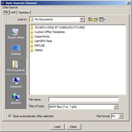
Figure 41: Data source chooser window
ScopeView can acquire data from many sources (Files of type). This section describes how to specify the data sources you want to use during a work session.
4.6.5.1. EMTP
The EMTP source allows importing signals saved previously in an .m, or .pl4, file generated by the EMTP simulation software.
4.6.5.2. MATLAB
The MATLAB source is used to import signals saved previously in a .mat file generated by the MATLAB processing software.
The .mat file must contain a list of vectors with at least one of these vectors representing the abscissa (or time axis).
4.6.5.3. COMTRADE
The COMTRADE source allows importing signals saved previously in a .cfg file generated under the COMTRADE format.
To load previously saved sources, click on the file you want.
Select the signal type tab (EMTP, Matlab etc.);
Select the file format in accordance with the type of work station you are using, PC or UNIX
Click the button. (The Load button moves the files in the available signals area.).
Below the Loaded Data Source box is the Signal Type identification. From the pull-down list, select the type of signal you want to study. The list corresponds to the sensors installed in your simulation software or the usable Database.
It is possible to select files from the Loaded Data Source box (scroll-down-list) in order to display or delete them. It is possible to remove a single file or Remove All the files from the list and, finally the user can reload all or replace a file.
Remember, it is possible to study signals from two or more different sources at the same time.
Below the Available Signals area, six cells and one button are present.
Single: Any selected (mouse click) signal will move automatically to the Selected signals list.
Multiple: Click the signals you want then click the Add Signals button to add signals to the Selected Signals. Multiple selection is possible by clicking and holding the CTRL key.
The Add Signals button will show only when the multiple option is selected.
Normal: ScopeView will display one signal per graph.
Superimposed: ScopeView will display two or more traces in the same graph (depending how many signals you have selected.
Grid or Log: ScopeView will display, according to the ticked box, either a graph with or without a grid. The other option is used to display a linear or a logarithmic graph in the X axis.
Grid or Log: ScopeView will display, according to the ticked box, either a graph with or without a grid. The other option is used to display a linear or a logarithmic graph in the Y axis.
Select the page number where you want to display the selected signal.
From the pull-down list select the function you want to apply to the selected signal. The list contains simple functions (one signal per argument).
Advance functions are available by clicking one of the buttons.
When Multiple Signal Selection Mode is used, this button will add the selected signals to the list at the bottom part of the Selected Signal area.
This area shows all the selected signals and their description. The two right hand columns are used to display or not the result on the page of your choice.
By default the Signal column displays and confirms the selection of different signals.
To edit a signal, click on its cell, type in your changes and, hit <ENTER>. You must press <ENTER> to commit the changes or <ESC> to cancel. Either of these actions will return user to the default mode.
The Description column shows the signal description (often the same as the signal name under the Signal column.
The Show column, when “ticked” , the signal will be acquired and displayed in ScopeView.
In Page column, the number written under this column tells ScopeView on what page to display the result from that signal.
The numbered column at the far left is use to show the background edit menu. Right click on the line you want to edit.
Scope View offers a split screen option to ease the multiple data source use. Simply click the mouse in the Signals area to see the background menu. You can split the area either horizontally or vertically. To revert to a single screen, click on Close View. Below is an example of horizontally split screen from the data sources loaded in two sections.
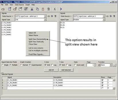
Figure 42: Signals form in split window option
The Remove button enables you to remove the current source or the Remove All button removes all the sources files from the scroll list.
To remove file (s) from the active list, display the source file you want to remove in the Loaded Data source file list;
Display the Data Source menu, and click on the Remove current data source item.
Or click on the Remove All button if desired.
If some formulas contain signals from a removed source, ScopeView displays a message asking to confirm this action. If you confirm, the formulas affected by the removal are automatically withdrawn from the list of formulas to evaluate.
The Replace button is used to change the characteristics of a source. This action is useful when you want to keep evaluating the same formulas, but with signals from a different source. The only restriction to replace a source is that the list of available signals should be the same.
To replace a source, in the Signal Form window, display the Data source menu;
Click on the source to change, select the Replace item.
ScopeView makes sure that the changes you make follow the replacement criteria. Otherwise, it refuses to execute the requested action.
The Signals section allows you to insert a new signal or function to the list of Selected Signals to evaluate.
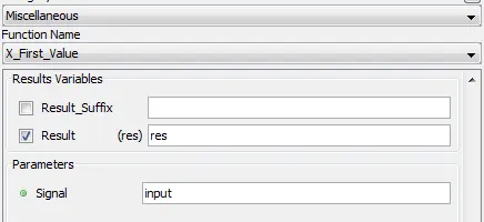
To apply an advance function to a signal, click on the name of the signal;
Select the category of function you want to apply to a signal (or select “All” to see all the available functions;
In the Function Name drop list, select a function;
Click the Add Function button.
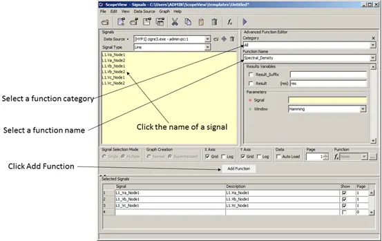
Figure 43: Signal form in advanced function option
The Simple Function (far right of the ScopeView – Signals form) section allows you to specify the mathematical operations to apply to the signals you select in the list of available signals. You can also configure other characteristics such as:
abs: absolute value;
acos: arc cosine
asin: arc sine
atan: arc tangent
cos: cosine
densp: spectral density
deriv: derivative
integ: integer
i2T: integral Time reverse sequence
log: logarithm
log10: logarithm base 10
min: minimum
max: maximum
moy: average
rms: root mean square
sin: sine
sqrt: square root
tan: tangent
To apply a simple function to a signal, select the mathematical function to be applied to a signal using the menu related to the Function item.
Select a signal; Click Add Signals button.
4.9.3. List of formulas to evaluate
The Selected Signals area contains the list of formulas to evaluate during the acquisition. Each line in the list describes a signal (and a function in some cases) to evaluate and specifies characteristics such as:
Description;
Show;
Page.
Initially, ScopeView displays the results in a graphic page corresponding to their appearance order in the list of Selected Signals. After a first acquisition, you can change the display order by displacing the graphs interactively.
The Selected Signal field specifies a formula to evaluate. A new formula can be generated automatically by ScopeView or built manually.
To insert automatically a new formula, click on the selected source in the Data Source list;
Click on the signal you want in the list of Signals.
Select the processing to be applied from the pull-down list under Function to apply;
To edit manually a formula, click in the Formula field of the formula to edit.
Type the formula.
If this formula reuses a signal from another formula, you can then enter manually the identifier that was assigned to it by ScopeView. However, if the formula contains signals, which are not yet part of other formulas, you must insert them as follows to allow ScopeView to assign an identifier to each new signal:
Click on the selected source in the list of Data sources.
Click on the Multiple Signal Selection Mode and the function to be applied from the pull-down list under Simple Function to apply.
Click on the name of the chosen signal in the list of Signals.
ScopeView has a formula interpreter to evaluate complex formulas. This interpreter supports the following operators and functions:
Standard arithmetic operators (+, -, *, /, ** or ^, vs);
Assigning in one or many variables that can be reused by other formulas;
Standard mathematical functions (sine, cosine, logarithm, etc.);
Internal functions for spectral analysis (spectral density, frequency response, etc.);
TYRAN functions (calculation of module and phase for a symmetric, integral component, etc.);
External functions for signal processing (calculation of fundamental frequency, harmonics, digital filters, etc.).
You can specify in the Description field the description to identify the result of the formula during graphic display.
ScopeView automatically generates a default description when inserting a new formula. This description consists of an abbreviation representing the mathematical operation applied to the signal and the signal name (or signals) selected.
The Show checkmark box specifies to ScopeView if it must display the formula result in a graph.
ScopeView automatically selects this item when a signal or a function is inserted from the list of Signals.
If you build manually a formula and you select this item, ScopeView will automatically initialize at 1 the Page field for the formula. You can change this page number if you wish.
The Page field specifies the destination graphic page for the formula.
4.9.7. Editing the list of formulas
The list of signals can be edited to change the display order of the formulas or to delete them from the list.
You can edit the list of formulas either using the menu associated with the Edit menu, or the background menu associated with the scroll list. This menu allows executing the following commands:
To select one signal only, click in the far left column beside the required signal.
Select all: to select all the formulas.
Select none: to unselect all the formulas.
Cut: To cut selected formulas and save them in the buffer
Copy: To copy selected formulas in the buffer
Paste: To add to the list formulas from the buffer
Delete: To remove selected formulas without affecting the content of the buffer
To cut one or more formulas, move your cursor in the far left column and right click to display the background menu.
Click on Cut to cut and save in the buffer.
To copy one or more formulas, move your cursor in the far left column and right click to display the background menu.
Select the Copy option from the Edit menu.
To paste the content of the buffer, move your cursor in the far left column and right click to display the background menu.
Select paste the content of the buffer:
To delete one or more formulas, move your cursor in the far left column and right click to display the background menu.
Select the Delete option from the background menu.
In order to accelerate the configuration of repetitive and identical acquisitions from one session to another, ScopeView allows you to save and retrieve the information on the formulas to evaluate.
The following information is contained in a template acquisition:
List of sources used;
Acquisition numbers;
List of signals to acquire;
List of formulas to evaluate;
Editing information (number of columns, superimposition, zoom, etc.)
You can load a previously saved template acquisition by selecting the button or the Open Template... item in the File menu. The software displays the form to select the file to open. The scroll list allows navigating in the file tree-structure.
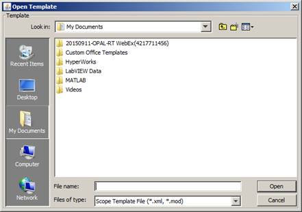
Figure 44: Open template window
To load a template acquisition, click on the button or from the File menu click on Open Template...
In the scroll list, select the template acquisition wanted.
Click on the Open... button.
4.11.1.1. Number of Acquisition
The Number of Acquisition field specifies the number of acquisitions to be executed by ScopeView.
If the signals originate from acquisition units, it can be useful to have a number of acquisitions higher than one to see the evolution of the acquisition signals from one acquisition to another or to compute the average of the results obtained.
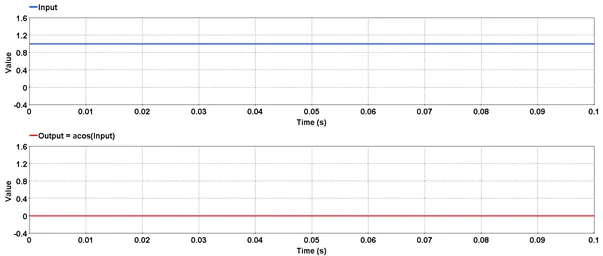
Outputs the arc cosine value of the input.
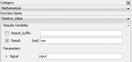
5.1.1.1. Category
Trigonometric
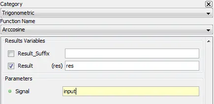
5.1.1.2. Description
Outputs the inverse cosine or arc cosine value of the input. The output value is in radians.
5.1.1.3. Result Variables and Parameters
Result: Arc cosine value [radians]
Signal: Cosine value
5.1.1.4. Syntax
res = acos(input)
5.1.1.5. Characteristics
|
Data type support |
Double Floating point |
5.1.1.6. Example
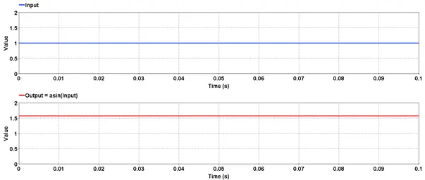
Outputs the arc sine value of the input.
5.1.2.1. Category
Trigonometric
5.1.2.2. Description
Outputs the inverse sine or arc sine value of the input. The output value is in radians.
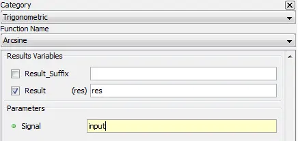
5.1.2.3. Result Variables and Parameters
Result: Arc sine value [radians]
Signal: Sine value
5.1.2.4. Syntax
res = asin(input)
5.1.2.5. Characteristics
|
Data type support |
Double Floating point |
5.1.2.6. Example
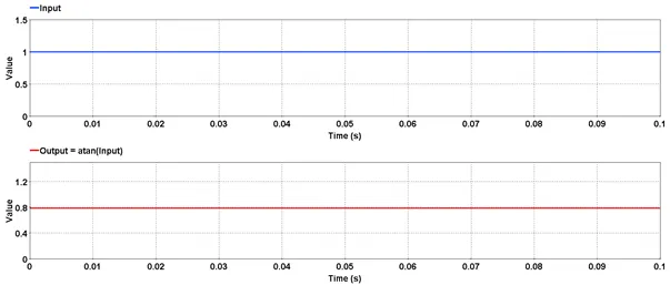
Outputs the arc tangent value of the input.
5.1.3.1. Category
Trigonometric
5.1.3.2. Description
Outputs the inverse tangent or arc tangent value of the input. The output value is in radians.
5.1.3.3. Result Variables and Parameters
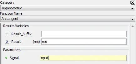
Result: Arc tangent value [radians]
Signal: Tan value
5.1.3.4. Syntax
res=atan(input)
5.1.3.5. Characteristics
|
Data type support |
Double Floating point |
5.1.3.6. Example
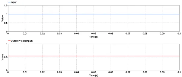
Outputs the cosinusoidal value of the input.
5.1.4.1. Category
Trigonometric
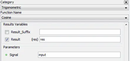
5.1.4.2. Description
Outputs the cosinusoidal value of the input. The input value is in radians.
5.1.4.3. Result Variables and Parameters
Result: Cosine value
Signal: The input value [radians]
5.1.4.4. Syntax
res=cos(input)
5.1.4.5. Characteristics
|
Data type support |
Double Floating point |
5.1.4.6. Example
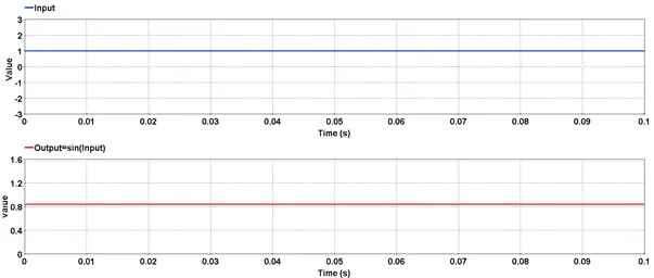
Outputs the sinusoidal value of the input.
5.1.5.1. Category
Trigonometric
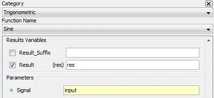
5.1.5.2. Description
Outputs the sinusoidal value of the input. The input value is in radians.
5.1.5.3. Result Variables and Parameters
Result: Sine value
Signal: The input value [radians]
5.1.5.4. Syntax
Res=sin(input)
5.1.5.5. Characteristics
|
Data type support |
Double Floating point |
5.1.5.6. Example
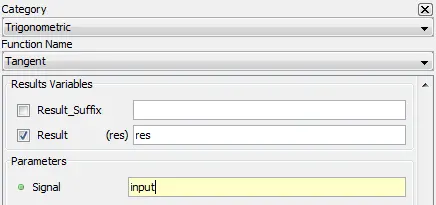
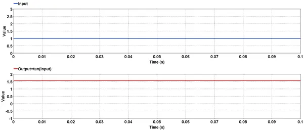
Outputs the tangent value of input.
5.1.6.1. Category
Trigonometric
5.1.6.2. Description
Outputs the tangent value of input. The input value is in radians.
5.1.6.3. Result Variables and Parameters
Result: Tangent value
Signal: The input value [radians]
5.1.6.4. Syntax
res=tan(input)
5.1.6.5. Characteristics
|
Data type support |
Double Floating point |
5.1.6.6. Example
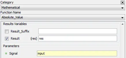
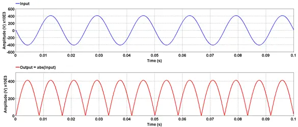
Outputs the absolute value of selected signal.
5.2.1.1. Category
Mathematical
5.2.1.2. Description
Outputs the absolute value of selected signal.
5.2.1.3. Result Variables and Parameters
Result: Absolute value
Signal: Input
5.2.1.4. Syntax
res=abs(input)
5.2.1.5. Characteristics
|
Data type support |
Double Floating point |
5.2.1.6. Example
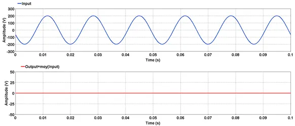
Outputs the average value of the input.
5.2.2.1. Category
Mathematical
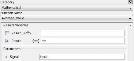
5.2.2.2. Description
Outputs the average value of the input over one acquisition.
5.2.2.3. Result Variables and Parameters
Signal: Input
Result: Average value
5.2.2.4. Syntax
res=moy(input)
* Moyenne is a French word meaning average.
5.2.2.5. Characteristics
|
Data type support |
Double Floating point |
5.2.2.6. Example
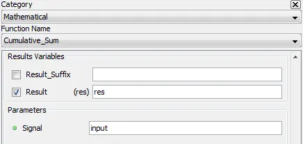
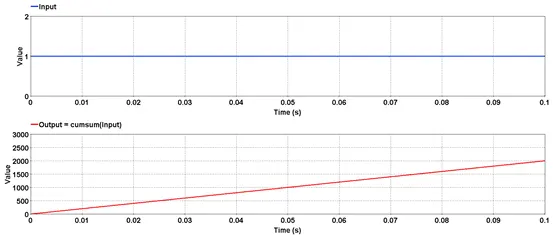
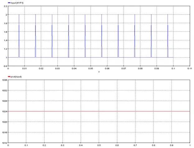
5.2.3. Cumulative sum – [cumsum]
Outputs the cumulative sum of input over time.
5.2.3.1. Category
Mathematical
5.2.3.2. Description
Outputs the cumulative sum of input over time.
5.2.3.3. Result Variables and Parameters
Result: Cumulative sum
Signal: Input
5.2.3.4. Syntax
res=cumsum(input)
5.2.3.5. Characteristics
|
Data type support |
Double Floating point |
5.2.3.6. Example
In the below example, a signal of constant value of 1 is given as input to the function cumsum. The sampling frequency is set at 20000 samples/second. Thus, in a duration of 0.1 second, there will be 2000 sample points. Thus, output of the function is the sum of 1 over each sampling period. At the end of 0.1 second, the output value will be 2000.
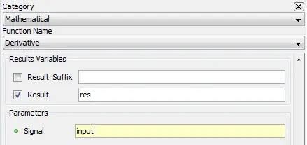
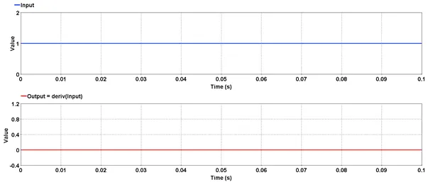
Outputs the derivative of the input.
5.2.4.1. Category
Mathematical
5.2.4.2. Description
Outputs the derivative or the slope of the input.
5.2.4.3. Result Variables and Parameters
Result: Derivative of the input
Signal: Input
5.2.4.4. Syntax
res=deriv(input)
5.2.4.5. Characteristics
|
Data type support |
Double Floating point |
5.2.4.6. Example
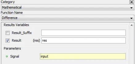
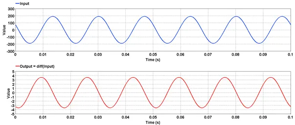
Outputs the difference between two consecutive samples from the input.
5.2.5.1. Category
Mathematical
5.2.5.2. Description
Outputs the difference between two consecutive samples from the input. Output will always have one sample point less than the input as there will be no output sample corresponding to first input sample.
5.2.5.3. Result Variables and Parameters
Result: Difference of the input
Signal: Input
5.2.5.4. Syntax
res=diff(input)
5.2.5.5. Characteristics
|
Data type support |
Double Floating point |
|
Output Size |
If [N] is the size of the input signal, the size of output signal is [N-1]. |
5.2.5.6. Example
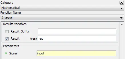
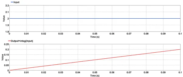
Outputs the integral of the input.
5.2.6.1. Category
Mathematical
5.2.6.2. Description
Outputs the integral of the input.
5.2.6.3. Result Variables and Parameters
Result: Integral of the input
Signal: Input
5.2.6.4. Syntax
res=integ(input)
5.2.6.5. Characteristics
|
Data type support |
Double Floating point |
5.2.6.6. Example
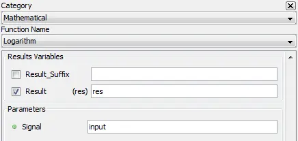
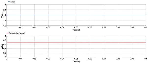
Outputs the natural logrithm of input.
5.2.7.1. Category
Mathematical
5.2.7.2. Description
Outputs the natural logrithm of input.
5.2.7.3. Result Variables and Parameters
Result: Logarithm of input
Signal: Input
5.2.7.4. Syntax
res=log(input)
5.2.7.5. Characteristics
|
Data type support |
Double Floating point |
5.2.7.6. Example
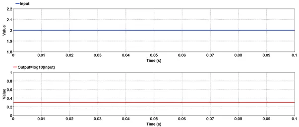
Outputs logrithm to the base 10 of input.
5.2.8.1. Category
Mathematical
5.2.8.2. Description
Outputs logrithm to the base 10 of input.
5.2.8.3. Result Variables and Parameters
Result: Logarithm of input
Signal: Input
5.2.8.4. Syntax
res=log10(input)
5.2.8.5. Characteristics
|
Data type support |
Double Floating point |
5.2.8.6. Example
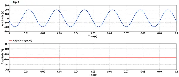
Outputs the maximum value of input.
5.2.9.1. Category
Mathematical
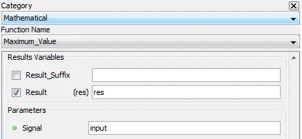
5.2.9.2. Description
Outputs the maximum value of input.
5.2.9.3. Result Variables and Parameters
Result: Maximum value of input
Signal: Input
5.2.9.4. Syntax
res=max(input)
5.2.9.5. Characteristics
|
Data type support |
Double Floating point |
5.2.9.6. Example
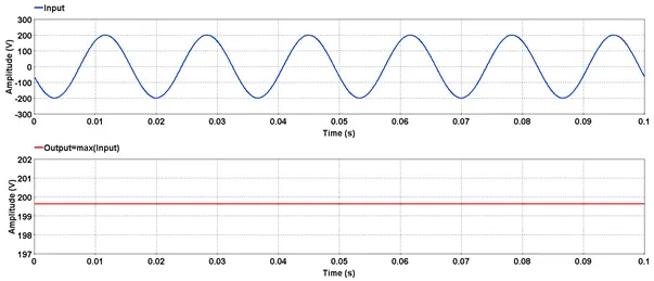
Outputs the minimum value of input.
5.2.10.1. Category
Mathematical
5.2.10.2. Description
Outputs the minimum value of input.
5.2.10.3. Result Variables and Parameters
Result: Minimum value of input
Signal: Input
5.2.10.4. Syntax
res=min(input)
5.2.10.5. Characteristics
|
Data type support |
Double Floating point |
5.2.10.6. Example
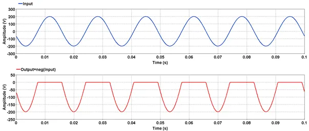
Outputs the negative values.
5.2.11.1. Category
Mathematical
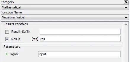
5.2.11.2. Description
Outputs the negative values. All values greater than zero are clamped to zero.
5.2.11.3. Result Variables and Parameters
Result: Negative value signal
Signal: Input
5.2.11.4. Syntax
res=neg(input)
5.2.11.5. Characteristics
|
Data type support |
Double Floating point |
5.2.11.6. Example
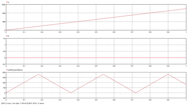
5.2.12. Phase Difference – [phasediff]
Outputs the absolute difference between two phases.
5.2.12.1. Category
Mathematical
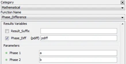
5.2.12.2. Description
Outputs the absolute diffence between two phases in degrees. Output is always between 0 and 180 degrees.
5.2.12.3. Result Variables and Parameters
Phase_Diff: Phase differences [degrees]
Phase 1: Phase 1 [degrees]
Phase 2: Phase 2 [degrees]
5.2.12.4. Syntax
pdiff=phasediff(phase1,phase2)
5.2.12.5. Characteristics
|
Data type support |
Double Floating point |
5.2.12.6. Example
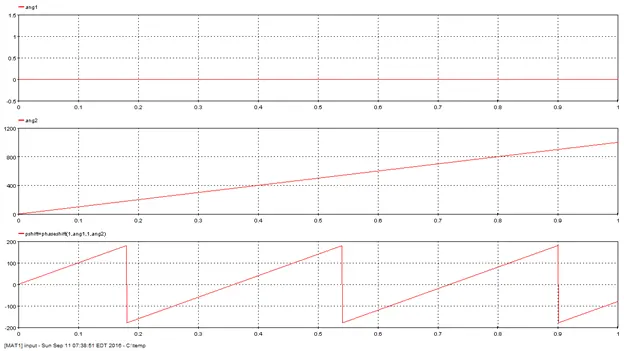
5.2.13. Phase shift – [phaseshift]
Outputs the phase difference between two vectors in degrees.
5.2.13.1. Category
Mathematical
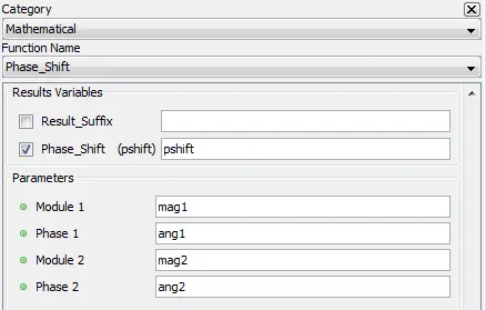
5.2.13.2. Description
Outputs the phase difference between two vectors in degrees. Output is always between -180 and 180 degrees. When modules(magnitudes) are negatives, it has the same effect as rotating the vector by 180 degrees.
5.2.13.3. Result Variables and Parameters
Phase_Shift: Phase difference [degrees]
Module 1 : Module of the first vector
Phase 1: Phase of the first vector [degrees]
Module 2 : Module of the second vector
Phase 2: Phase of the second vector [degrees]
5.2.13.4. Syntax
pshift=phaseshift(mag1,ang1,mag2,ang2)
5.2.13.5. Characteristics
|
Data type support |
Double Floating point |
5.2.13.6. Example
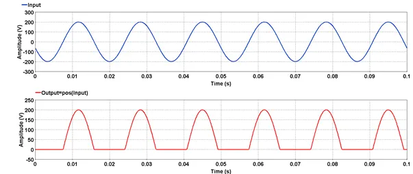
Outputs the positive values of input.
5.2.14.1. Category
Mathematical
5.2.14.2. Description
Outputs the positive values of input. All values lesser than zero are clamped to zero.
5.2.14.3. Result Variables and Parameters
Result: Positive value signal
Signal: Input
5.2.14.4. Syntax
res=pos(input)
5.2.14.5. Characteristics
|
Data type support |
Double Floating point |
5.2.14.6. Example
Outputs the product of all signal values
5.2.15.1. Category
Mathematical
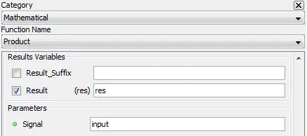
5.2.15.2. Description
Outputs the product of all input signal values, defined as:
![]()
were ![]() is the i-th signal value
is the i-th signal value
5.2.15.3. Result Variables and Parameters
Result: product of all input signal values
Signal: Input
5.2.15.4. Syntax
res=prod(input)
5.2.15.5. Characteristics
|
Data type support |
Double Floating point |
5.2.15.6. Example
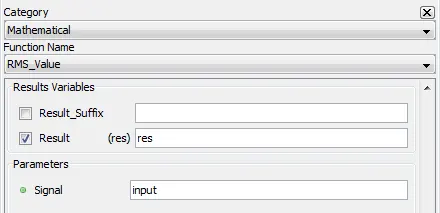
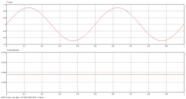
Outputs the root mean squate of the input signal.
5.2.16.1. Category
Mathematical
5.2.16.2. Description
Outputs the root mean square of the input signal.
5.2.16.3. Result Variables and Parameters
Result: Root mean square of the input
Signal: Input
5.2.16.4. Syntax
res=rms(input)
5.2.16.5. Characteristics
|
Data type support |
Double Floating point |
5.2.16.6. Example
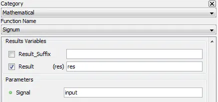
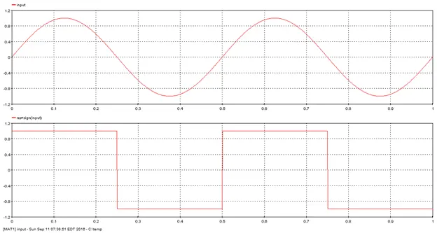
Outputs the sign of the input.
5.2.17.1. Category
Mathematical
5.2.17.2. Description
Outputs the sign of the input. Outputs 1 when input is greater than 0, -1 when input is less than 0, and 0 when input is 0.
5.2.17.3. Result Variables and Parameters
Result: Sign of input [-1, 0, 1].
Signal: Input
5.2.17.4. Syntax
res=sign(input)
5.2.17.5. Characteristics
|
Data type support |
Double Floating point |
5.2.17.6. Example
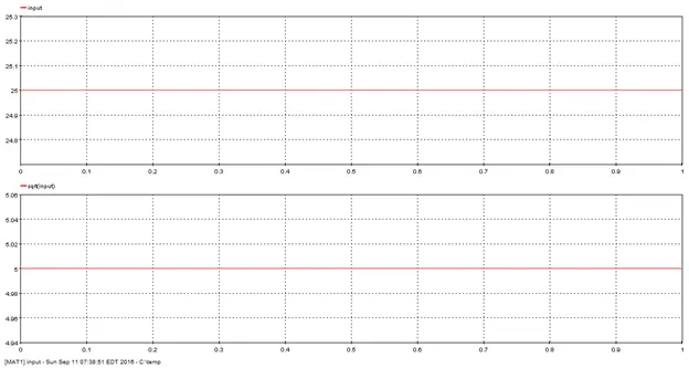
Outputs the square root of input
5.2.18.1. Category
Mathematical
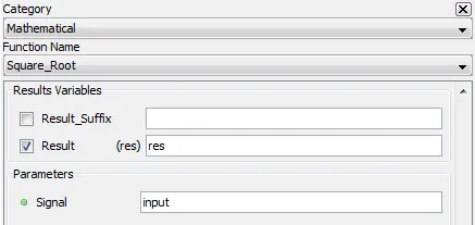
5.2.18.2. Description
Outputs the squate root of input
5.2.18.3. Result Variables and Parameters
Result: Square root of the input
Signal: Input
5.2.18.4. Syntax
res=sqrt(input)
5.2.18.5. Characteristics
|
Data type support |
Double Floating point |
5.2.18.6. Example
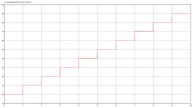
Generates discrete stairs at regular intervals .
5.2.19.1. Category
Mathematical
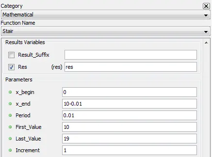
5.2.19.2. Description
Generates discrete stairs at regular intervals. The parameters x_begin, x_end, period, first_value, last_value and increment define the shape of the output. The following figure presents how to use each parameter.
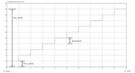
5.2.19.3. Result Variables and Parameters
Result: Stairs signal
x_begin: X minimum value
x_end: X maximum value
Period: time interval between X samples. The number of samples that output vector will contains is equal to (x_end-x_begin)/period+1.
First_Value: Y minimum value
Last_Value: Y maximum value
Increment: Y increment between stairs
5.2.19.4. Syntax
res=stair(x_begin,x_end,period,first_value,last_value,increment)
5.2.19.5. Characteristics
|
Data type support |
Double Floating point |
5.2.19.6. Example
Outputs the sum of all samples of input.
5.2.20.1. Category
Mathematical
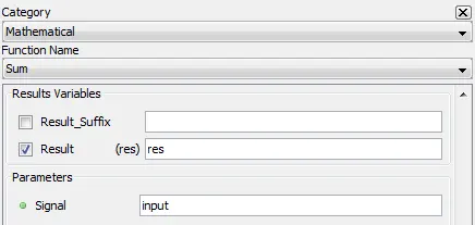
5.2.20.2. Description
Outputs the sum of all samples of input.
5.2.20.3. Result Variables and Parameters
Result: Sum of input
Signal: Input
5.2.20.4. Syntax
res=sum(input)
5.2.20.5. Characteristics
|
Data type support |
Double Floating point |
5.2.20.6. Example
For an input of value 1 acquired over a duration of 0.1 second at a sampling rate of 10000 Hz, the SUM function outputs the total sum of one thousand ones i.e. 1000. 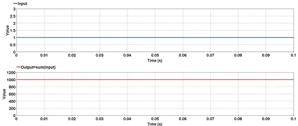
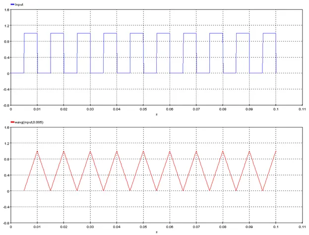
5.2.21. Window Average Value – [wavg]
Outputs the moving average of the input signal
5.2.21.1. Category
Mathematical
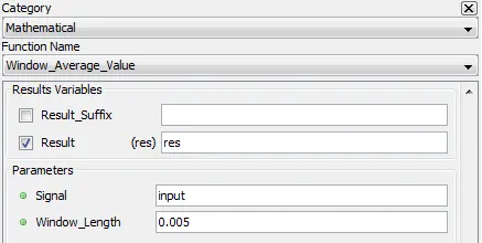
5.2.21.2. Description
Outputs the moving average of the input signal with a sliding window size defined by “Window_Length”.
5.2.21.3. Result Variables and Parameters
Result: Signal moving average
Signal: Input
Window_Length: Size of the sliding window in seconds
5.2.21.4. Syntax
res=wavg(Signal,Window_Length)
5.2.21.5. Characteristics
|
Data type support |
Double Floating point |
5.2.21.6. Example
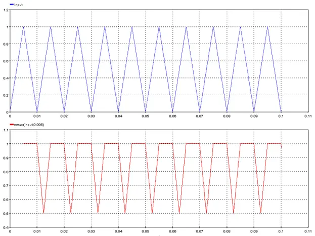
5.2.22. Window Maximum Value – [wmax]
Outputs the moving maximum of the input signal
5.2.22.1. Category
Mathematical
5.2.22.2. Description
Outputs the moving maximum of the input signal with a rolling window size defined by “Window_Length”.
5.2.22.3. Result Variables and Parameters
Result: Signal moving maximum
Signal: Input
Window_Length: Size of the rolling window in seconds
5.2.22.4. Syntax
res=wmax(input,Window_Length)
5.2.22.5. Characteristics
|
Data type support |
Double Floating point |
5.2.22.6. Example
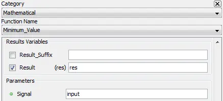
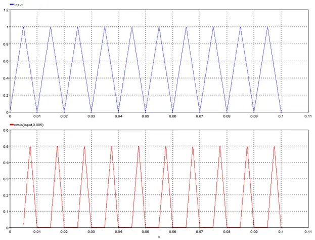
5.2.23. Window Minimum Value – [wmin]
Outputs the moving minimum of the input signal
5.2.23.1. Category
Mathematical
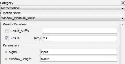
5.2.23.2. Description
Outputs the moving minimum of the input signal with a rolling window size defined by “Window_Length”.
5.2.23.3. Result Variables and Parameters
Result: Signal moving minimum
Signal: Input
Window_Length: Size of the rolling window in seconds
5.2.23.4. Syntax
res=wmin(input, Window_Length)
5.2.23.5. Characteristics
|
Data type support |
Double Floating point |
5.2.23.6. Example
5.2.24. Window RMS Value – [wrms]
Outputs the moving RMS of the input signal
5.2.24.1. Category
Mathematical
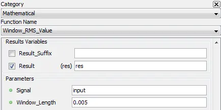
5.2.24.2. Description
Outputs the moving RMS of the input signal with a rolling window size defined by “Window_Length”.
5.2.24.3. Result Variables and Parameters
Result: Signal moving RMS
Signal: Input
Window_Length: Size of the rolling window in seconds
5.2.24.4. Syntax
res=wrms(input, Window_Length)
5.2.24.5. Characteristics
|
Data type support |
Double Floating point |
5.2.24.6. Example
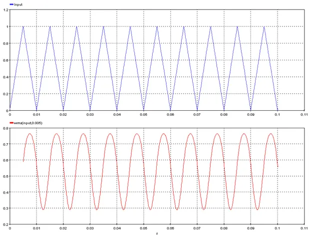
5.2.25. Window Sum Value – [wsum]
Outputs the moving sum of the input signal
5.2.25.1. Category
Mathematical
5.2.25.2. Description
Outputs the moving sum of the input signal with a rolling window size defined by “Window_Length”.
5.2.25.3. Result Variables and Parameters
Result: Signal moving sum
Signal: Input
Window_Length: Size of the rolling window in seconds
5.2.25.4. Syntax
res=wsum(input, Window_Length)
5.2.25.5. Characteristics
|
Data type support |
Double Floating point |
5.2.25.6. Example
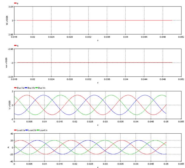
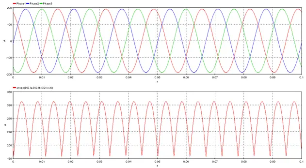
5.3.1. 3 Phase Power – [power3ph]
Computes the active and reactive power of a three phase element by using voltages and currents.
5.3.1.1. Category
Miscellaneous
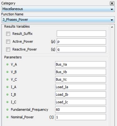
5.3.1.2. Description
This function allows to compute the active power and reactive power by using phase to ground voltages and currents signals. The inputs are transformed into direct sequence element and then the power is computed:
![]()
![]()
5.3.1.3. Result Variables and Parameters
Active Power: Active power of the input signals
Reactive Power: Reactive power of the input signals
V_A: Input voltage, phase A
V_B: Input voltage, phase B
V_C: Input voltage, phase C
I_A: Input current, phase A
I_B: Input current, phase B
I_C: Input current, phase C
Fundamental Frequency: Fundamental frequency of the inputs
Nominal Power: Nominal power of the network. This factor will divide the power displayed in ScopeView. Note that the unit of the graphic will not be updated.
5.3.1.4. Syntax
[p,q]=power3ph(Bus_Va,Bus_Vb,Bus_Vc,Load_Ia,Load_Ib,Load_Ic,60,1)
5.3.1.5. Characteristics
|
Data type support |
Double Floating point |
5.3.1.6. Example
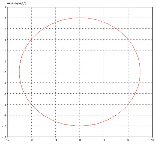
Outputs a circle
5.3.2.1. Category
Miscellaneous
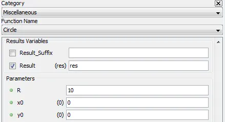
5.3.2.2. Description
Output a circle centered on [x0, y0] with radius R
5.3.2.3. Result Variables and Parameters
Result: circle centered on [x0, y0] with radius R
R: circle radius
x0: x coordinate of the circle center
y0: y coordinate of the circle center
5.3.2.4. Syntax
res=circle(R,x0,y0)
5.3.2.5. Characteristics
|
Data type support |
Double Floating point |
5.3.2.6. Example
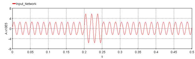
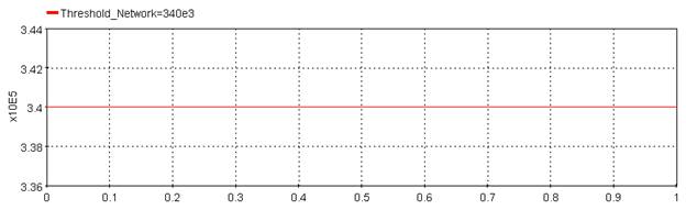
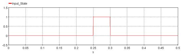
5.3.3. Clearing time – [clearingtime]
Outputs the clearing time by computing difference between a network signal and a state signal related to their respective threshold.
5.3.3.1. Category
Miscellaneous
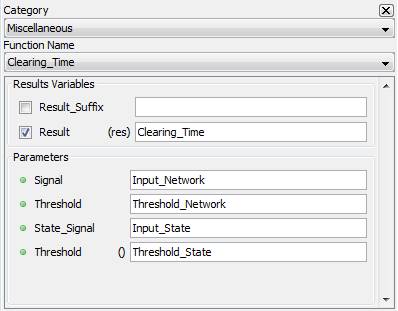
5.3.3.2. Description
Outputs the elapsed time between the two following events. The first event is the first positive slope zero crossing of the network signal before the threshold is reached. The threshold is compared to the Windowed RMS computation. The second event is when the state signal exceeds the threshold. Note that this function uses a windowed RMS computation set to a frequency of 60 Hz. The behaviour with a system using a different frequency can be different.
5.3.3.3. Result Variables and Parameters
Result: Clearing time [s]
Signal: Network signal input
Threshold: Network signal value threshold (RMS Value)
State Signal: State signal input
Threshold: State signal threshold
5.3.3.4. Syntax
Clearing_Time=clearingtime(Input_Network,Threshold_Network,Input_State,Threshold_State)
5.3.3.5. Characteristics
|
Data type support |
Double Floating point |
5.3.3.6. Example
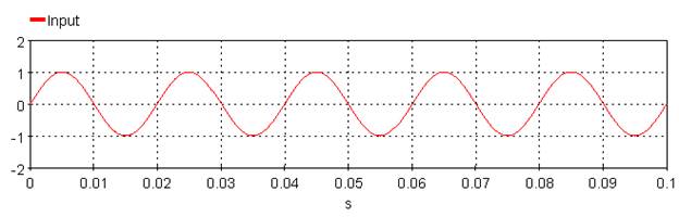
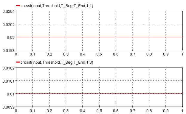
5.3.4. Crossing time – [crosst]
Output the time at which the signal cross the threshold depending on direction and slope parameter.
5.3.4.1. Category
Miscellaneous
5.3.4.2. Description
The function outputs time value at which the signal cross the threshold depending on direction and slope parameter. The scope of the search is limited to the window formed by Begin_Time and End_Time. Using HUGE for the End_Time will set the parameter to match the end of acquisition. If there is no match, the graphic will be empty.
Direction : Forward will search the threshold value from Begin_Time toward End_Time. Backward will do the opposite.
Slope : Using Positive Slope will search the threshold when the slope increase in function of time while Negative will search it when the slope decrease in function of time.
5.3.4.3. Result Variables and Parameters
Result: Time at which the signal cross the threshold in function of the parameters
Signal: Input signal
Threshold: Reference value to which the signal is compared
Begin Time: Beginning time of the function
End Time: Ending time of the function
Direction : Direction for the search (1: Forward, 0 : Backward)
Slope : Type of slope (1: Positive, 0 : Negative)
5.3.4.4. Syntax
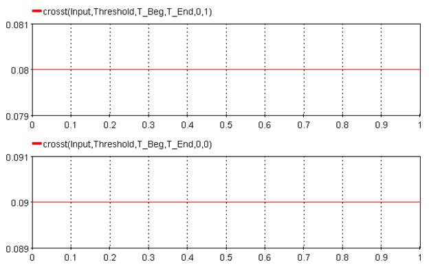
Result = crosst(Input,Threshold,T_Beg,T_End,Direction,Slope)
5.3.4.5. Characteristics
|
Data type support |
Double Floating point |
5.3.4.6. Example
Threshold = 0, T_Beg = 0, T_End = Huge
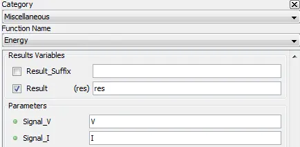
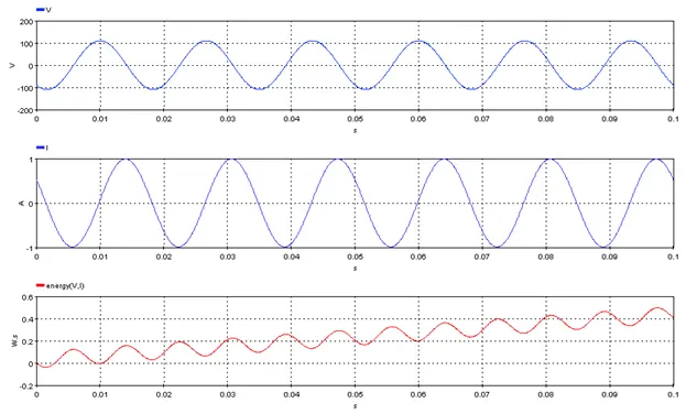
Outputs the energy corresponding to an input voltage and current
5.3.5.1. Category
Miscellaneous
5.3.5.2. Description
Outputs the energy corresponding to an input voltage Signal_V and current Signal_I. The energy is given by:
![]()
5.3.5.3. Result Variables and Parameters
Result: Energy (W.s / J)
Signal_V: Input voltage
Signal_I: Input current
5.3.5.4. Syntax
res=energy(Signal_V,Signal_I)
5.3.5.5. Characteristics
|
Data type support |
Double Floating point |
5.3.5.6. Example
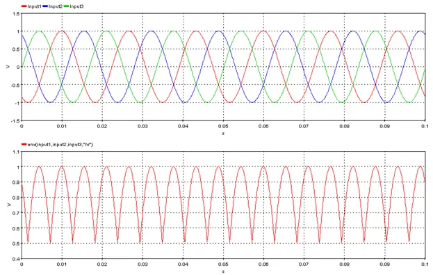
Outputs the upper, lower or absolute envelope of a set of three input signals
5.3.6.1. Category
Miscellaneous
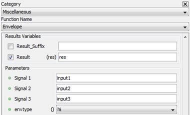
5.3.6.2. Description
Outputs the upper (hi), lower (lo) or absolute (abs) envelope of a set of three input signals given by:
![]() , for the upper envelope
, for the upper envelope
![]() , for the lower envelope
, for the lower envelope
![]() , for the absolute envelope
, for the absolute envelope
5.3.6.3. Result Variables and Parameters
Result: Upper lower or absolute envelope
Signal1: input1
Signal2: input1
Signal3: input1
envtype: Type of the envelope, lower (lo), upper (hi), absolute (abs).
5.3.6.4. Syntax
res = env(Signal1,Signal2,Signal3,envtype)
5.3.6.5. Characteristics
|
Data type support |
Double Floating point |
5.3.6.6. Example
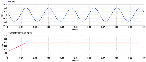
5.3.7. Peak of Envelop – [envpeak]
Outputs the peak value of the input (peak of envelope). The function displays output only if the next sample of the input is greater than or equal to previous peak identified.
5.3.7.1. Category
Miscellaneous
5.3.7.2. Description
Outputs the peak value of the input (peak of envelope). The function displays output only if the next sample of the input is greater than or equal to previous peak identified.
5.3.7.3. Result Variables and Parameters
Result: Peak value of the input
Signal: Input
5.3.7.4. Syntax
res=envpeak(input)
5.3.7.5. Characteristics
|
Data type support |
Double Floating point |
5.3.7.6. Example
Consider a sinusoidal signal with a periodicity of 16.67 ms (60 Hz) as input. Over a duration of 0.1 second, there will be 6 peaks. The function will have exactly 7 output points corresponding to 6 peaks and one for the first sample. That is because the function will detect only a positive peak and display only if the detected peak is either greater or equal to the previous peak value.
In the below example, though the output seems to be continuous, it is only because an inherent linear interpolation algorithm is used between two successive peaks. For the same reason, there is no output graph visible after the last peak (around 0.095 second).
5.3.8. Envelope Phase–Phase – [envpp]
Outputs the envelope of the phase-to-phase differences of a 3-phase signal
5.3.8.1. Category
Miscellaneous
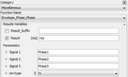
5.3.8.2. Description
Outputs the upper (hi), lower (lo) or absolute (abs) of the phase-to-phase differences of a 3-phase signal:
![]() ,
,
for the upper envelope
![]() ,
,
for the lower envelope
![]() ,
,
for the absolute envelope
5.3.8.3. Result Variables and Parameters
Result: Upper lower or absolute phase-to-phase envelope
Signal1: Phase1
Signal2: Phase2
Signal3: Phase3
envtype: Type of the envelope, lower (lo), upper (hi), absolute (abs).
5.3.8.4. Syntax
res = envpp(Signal1,Signal2,Signal3,envtype)
5.3.8.5. Characteristics
|
Data type support |
Double Floating point |
5.3.8.6. Example
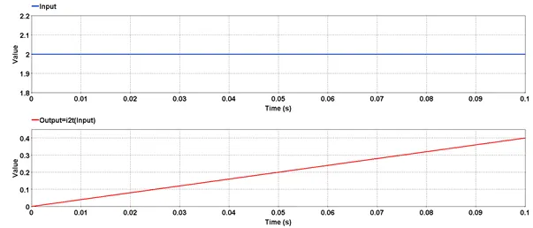
5.3.9. Product of time step and square of the input – [I2T]
Outputs the product of the simulation time step and square of the input signal.
5.3.9.1. Category
Miscellaneous
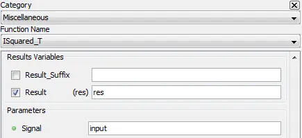
5.3.9.2. Description
Outputs the product of simulation time step and square of the input signal.
5.3.9.3. Result Variables and Parameters
Result: Product
Signal: Input
5.3.9.4. Syntax
res = i2t(input)
5.3.9.5. Characteristics
|
Data type support |
Double Floating point |
5.3.9.6. Example
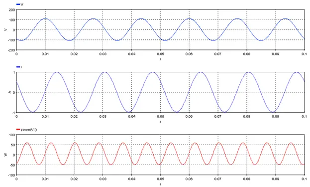
5.3.10. Instantaneous Power – [Power]
Outputs the instantaneous power of an input voltage and current
5.3.10.1. Category
Miscellaneous
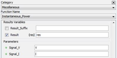
5.3.10.2. Description
Outputs the instantaneous power of an input voltage Signal_V and current Signal_I. The instantaneous power is given by:
![]()
5.3.10.3. Result Variables and Parameters
Result: Instantaneous_Power (W)
Signal_V: Input voltage
Signal_I: Input current
5.3.10.4. Syntax
res=power(Signal_V,Signal_I)
5.3.10.5. Characteristics
|
Data type support |
Double Floating point |
5.3.10.6. Example
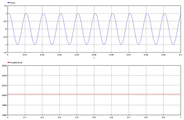
Outputs the number of samples of the input signal
5.3.11.1. Category
Miscellaneous
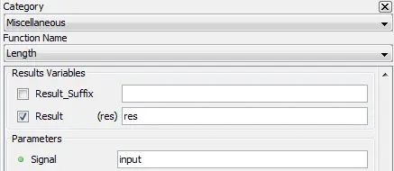
5.3.11.2. Description
Outputs the number of samples of the input signal
5.3.11.3. Result Variables and Parameters
Result: Number of samples
Signal: Input
5.3.11.4. Syntax
res=length(Signal)
5.3.11.5. Characteristics
|
Data type support |
Double Floating point |
5.3.11.6. Example
Outputs the input signal over a given range
5.3.12.1. Category
Miscellaneous
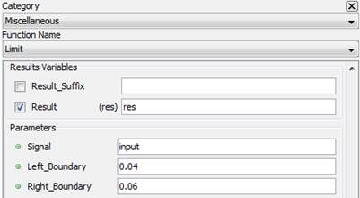
5.3.12.2. Description
Outputs the input signal Signal over a range given by Left_Boundary and Right_Boundary
5.3.12.3. Result Variables and Parameters
Result: Signal in the range [Left_Boundary, Right_Boundary]
Signal: Input
Left_Boundary: Left boundary of the output range
Right_Boundary: Right boundary of the output range
5.3.12.4. Syntax
res=lim(Signal,Left_Boundary,Right_Boundary)
5.3.12.5. Characteristics
|
Data type support |
Double Floating point |
5.3.12.6. Example
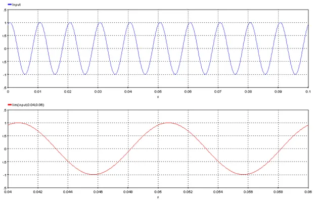
5.3.13. Maximum Finite Value – [maxf]
Outputs the maximum finite value of the input signal
5.3.13.1. Category
Miscellaneous
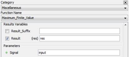
5.3.13.2. Description
Outputs the maximum finite value of the input signal
5.3.13.3. Result Variables and Parameters
Result: maximum finite value of the input signal
Signal: Input
5.3.13.4. Syntax
res=maxf(Signal)
5.3.13.5. Characteristics
|
Data type support |
Double Floating point |
5.3.13.6. Example
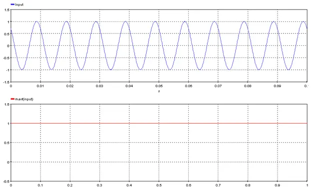
5.3.14. Minimum Finite Value – [minf]
Outputs the minimum finite value of the input signal
5.3.14.1. Category
Miscellaneous
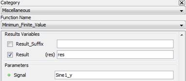
5.3.14.2. Description
Outputs the minimum finite value of the input signal
5.3.14.3. Result Variables and Parameters
Result: minimum finite value of the input signal
Signal: Input
5.3.14.4. Syntax
res=minf(Signal)
5.3.14.5. Characteristics
|
Data type support |
Double Floating point |
5.3.14.6. Example
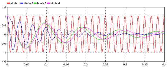
5.3.15. Modal analysis – [amod]
This functions output modal analysis of a single input signal.
5.3.15.1. Category
Miscellaneous
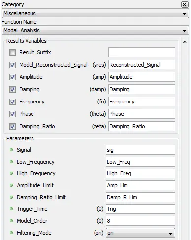
5.3.15.2. Description
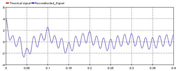
The modal analysis returns the dynamic parameters containing the amplitude, damping, frequency, phase shift and damping ratio of each complex mode identified in the input signal by processing it through an ERA/Prony algorithm method.
To return the modal analysis results, the analyzed input signal is presumed as the impulse-response of a black-box dynamic state-space system. The system identification of this dynamic system is obtained by applying the Eigensystem realization algorithm (ERA) based on Hankel matrices, singular value decomposition and Markov parameters calculation to the input signal. From this system identification, the Prony approach algorithm is then applied to obtain the dynamic parameters based on the system’s equation and residual terms calculation.
5.3.15.3. Result Variables and Parameters
Model Reconstructed Signal: Input signal reconstructed with the dynamic parameters from the k complex mode identified in the analysis
Amplitude: Modal amplitude [ak]
Damping: Modal damping value [σk]
Frequency: Modal frequency [fk]
Phase: Phase shift [ϴk]
Damping Ratio: Modal relative damping ratio [ζk]
Signal: Input signal to be analyzed
Low Frequency: Low frequency limit for oscillatory modes for the input signal. This limit must be set so there is at least a complete period in the window selected for analysis.
It must respect the following : ![]()
High Frequency: High frequency limit for oscillatory modes for the input signal. It must be define in a way so undersampling is avoided : ![]()
Amplitude Limit: Proportional maximum between the highest and lowest amplitudes of oscillatory mode displayed.
![]()
![]()
Damping Ratio Limit: Minimum relative damping of oscillatory modes displayed.
![]()
Trigger Time: Time at which the analysis begin. It must be determined in a way that at least a period of Low Frequency is observable. The starting time will be floored to the first sample available.
Model Order: Number of elements kept for the minimal realization of ERA.
0: Model order is automatically set with the singular values decomposition evaluation of the Hankel matrix.
Greater than 0: Model order is manually set to this value. However if the chosen order is greater than the maximal order permitted for the computation of Hankel matrix, the order will be set automatically.
Filtering Mode (optional) [On =1 , Off = 0]: Define if bandpass filter is applied or not. Low and High Frequency parameters will define the cutoff frequencies.
5.3.15.4. Syntax
[Reconstructed_Signal,Amplitude,Damping,Frequency,Phase,Damping_Ratio]=amod(sig,Low_Freq,High_Freq,Amp_Lim,Damp_R_Lim,Trig,8,0)
Note that 8 is the Order and 0 is the filter. Since these only accept integer value, parameters cannot be set by variable.
5.3.15.5. Characteristics
|
Data type support |
Double Floating point Integer for Model Order and Filtering Mode |
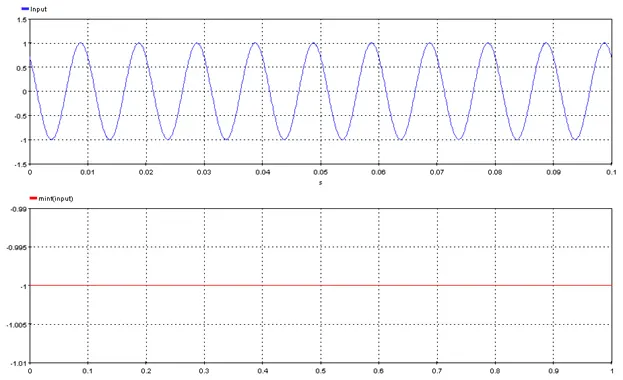
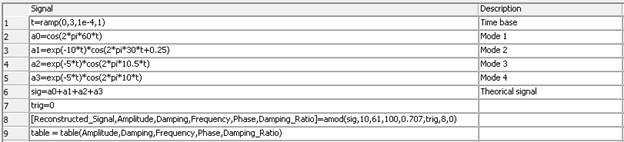
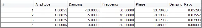
5.3.15.6. Example
For this example, a simple signal is constructed with ScopeView
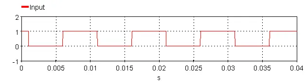
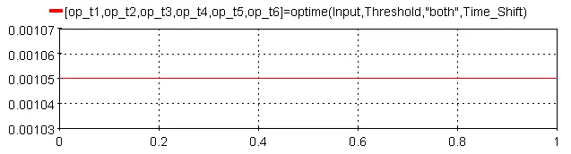
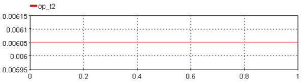
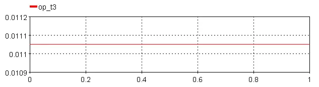
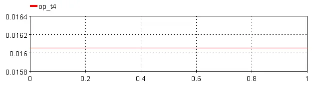
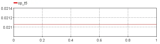
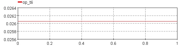
5.3.16. Operation Time – [optime]
Returns up to 6 time values crossing the threshold in function of the direction selection.
5.3.16.1. Category
Miscellaneous
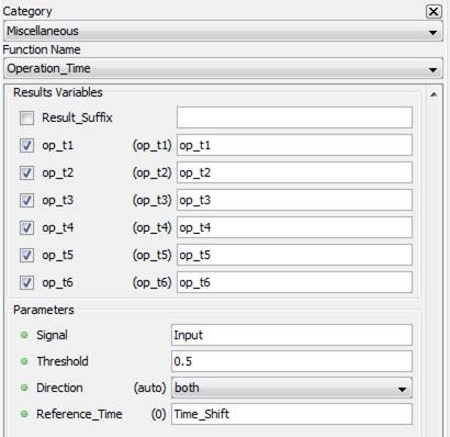
5.3.16.2. Description
Returns up to 6 time values crossing the threshold in function of the direction selection. Note that “auto” selection in Direction will select “rising” if the signal at t=0 is lower than the threshold and “falling” if the signal is higher than the threshold.
5.3.16.3. Result Variables and Parameters
Result:
op_t1: Output time 1
op_t2: Output time 2
op_t3: Output time 3
op_t4: Output time 4
op_t5: Output time 5
op_t6: Output time 6
Parameters:
Signal: Input signal
Threshold: Threshold used to compare the input signal and return the output time
Direction: [“auto”] : If input(0) >= Threshold, Direction = “falling”. If input(0) < Threshold, Direction = “rising”
[“rising”] : Output time will be the first six rising edge that cross the threshold
[“falling”] : Output time will be the first six falling edge that cross the threshold
[“both”] : Output time will be the first six rising and falling edge that cross the threshold
Reference Time: The output time is represented by the crossing time shifted by the reference time. If the first crossing occurs at t=1.0 and Reference Time = 0.25, op_t1 will be 0.75.
5.3.16.4. Syntax
[op_t1,op_t2,op_t3,op_t4,op_t5,op_t6]=optime(Input,Threshold,"both",Time_Shift)
5.3.16.5. Characteristics
|
Data type support |
Double Floating point |
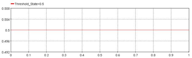
5.3.16.6. Example
Where Threshold = 0.5 and Time_Shift = 0
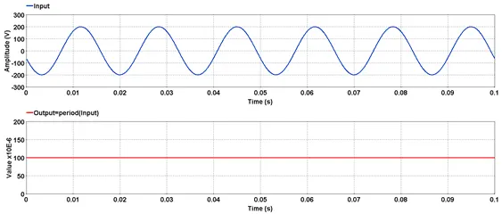
Outputs sample period used for data acquisition.
5.3.17.1. Category
Miscellaneous
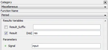
5.3.17.2. Description
Outputs sample period used for data acquisition of the selected input in microseconds.
5.3.17.3. Result Variables and Parameters
Result: Sample period [µs]
Signal: Input
5.3.17.4. Syntax
res=period(input)
5.3.17.5. Characteristics
|
Data type support |
Double Floating point |
5.3.17.6. Example
A sine wave was acquired with a sampling rate of 10000 Hz. The period corresponding to acquisition is 100 µs.
Outputs a ramp function
5.3.18.1. Category
Miscellaneous
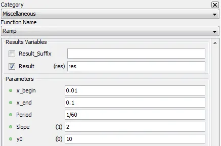
5.3.18.2. Description
Outputs a ramp function between between x_begin and x_end with period Period, slope Slope and ordinate at x_begin y0.
5.3.18.3. Result Variables and Parameters
Result: Sampling rate [Hz]
Signal: Input
5.3.18.4. Syntax
res=rate(input)
5.3.18.5. Characteristics
|
Data type support |
Double Floating point |
5.3.18.6. Example
Outputs the acquisition sampling rate.
5.3.19.1. Category
Miscellaneous
5.3.19.2. Description
Outputs the acquisition sampling rate of the selected input in Hertz [Hz]. This is same value as the one defined in ScopeView Acquisition Parameters.
5.3.19.3. Result Variables and Parameters
Result: Sampling rate [Hz]
Signal: Input
5.3.19.4. Syntax
res=rate(input)
5.3.19.5. Characteristics
|
Data type support |
Double Floating point |
5.3.19.6. Example
![]() A sine wave acquired at a sampling frequency of 10000 Hz is shown below.
A sine wave acquired at a sampling frequency of 10000 Hz is shown below.
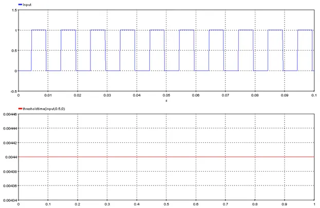
5.3.20. Threshold Time – [thresholdtime]
Outputs the time where the input signal value pass a given threshold
5.3.20.1. Category
Miscellaneous
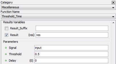
5.3.20.2. Description
Outputs the time where the input signal value pass a given threshold Threshold, with an optional additional delay Delay
5.3.20.3. Result Variables and Parameters
Result: Threshold time
Signal: Input
Threshold: threshold value
Delay: Optional delay value
5.3.20.4. Syntax
res= thresholdtime(Signal,Threshold,Delay)
5.3.20.5. Characteristics
|
Data type support |
Double Floating point |
5.3.20.6. Example
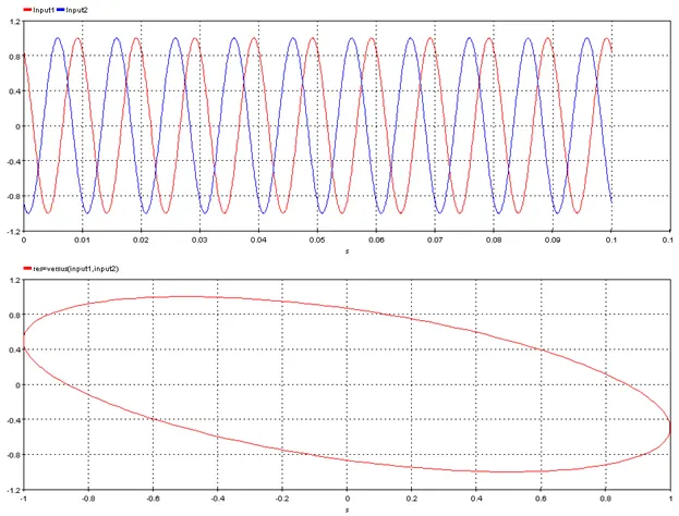
Outputs one signal vs another signal
5.3.21.1. Category
Miscellaneous
5.3.21.2. Description
Outputs one signal vs another signal
5.3.21.3. Result Variables and Parameters
Signal X: abscissa signal
Signal Y: ordinate signal
5.3.21.4. Syntax
res= versus(input1,input2)
res = input1 vs input2
5.3.21.5. Characteristics
|
Data type support |
Double Floating point |
5.3.21.6. Example
Outputs the sampling time of the first data in the acquisition buffer.
5.3.22.1. Category
Miscellaneous
5.3.22.2. Description
Outputs the sampling time of the first data of the input stored in the acquisition buffer in seconds [s].
5.3.22.3. Result Variables and Parameters
Result: Sampling time of the first data [s]
Signal: Input
5.3.22.4. Syntax
res = xfirst(input)
5.3.22.5. Characteristics
|
Data type support |
Double Floating point |
5.3.22.6. Example
In the below example, acquisition is started exactly at the same time as the trigger condition (without time offset). Sampling time of the first data is then 0 second.
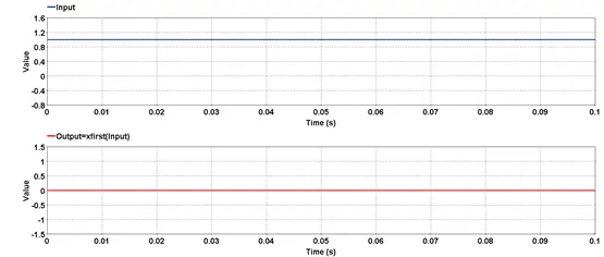
Outputs the sampling time of the last data in the acquisition buffer.
5.3.23.1. Category
Miscellaneous
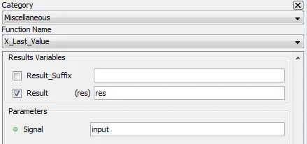
5.3.23.2. Description
Outputs the sampling time of the last data of the input stored in the acquisition buffer in seconds [s].
5.3.23.3. Result Variables and Parameters
Result: Sampling time of the last data [s]
Signal: Input
5.3.23.4. Syntax
res = xlast(input)
5.3.23.5. Characteristics
|
Data type support |
Double Floating point |
5.3.23.6. Example
In the below example, acquisition is started exactly at the same time as the trigger condition (without time offset) and the acquisition time length is 0.1 second. Sampling time of the last data is then 0.1 second.
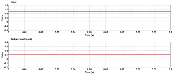
Outputs the input signal with a time shift.
5.3.24.1. Category
Miscellaneous
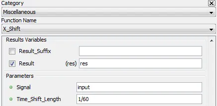
5.3.24.2. Description
Outputs the input signal (Signal) with a time shift (Time_Shift_Length)
5.3.24.3. Result Variables and Parameters
Signal: input signal
Time_Shift_Lenght: length of the time shift in seconds
5.3.24.4. Syntax
res = xshift(input,1/60)
5.3.24.5. Characteristics
|
Data type support |
Double Floating point |
5.3.24.6. Example
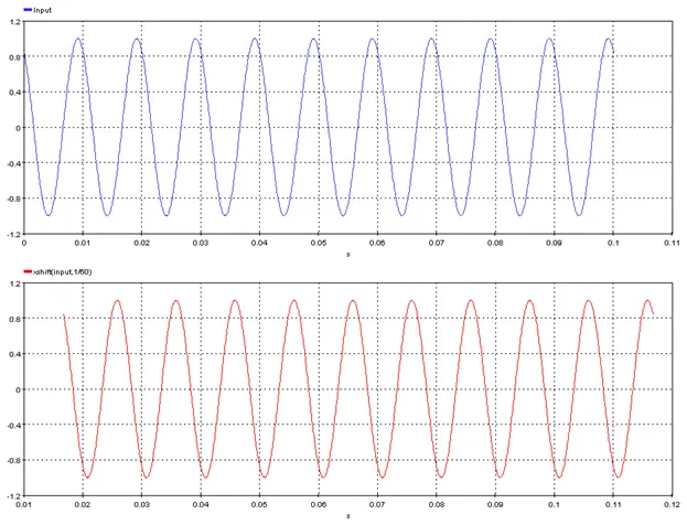
5.4.1. Cumulative Probability – [cumprob]
Outputs the cummulative distribution function of a signal
5.4.1.1. Category
Statistical
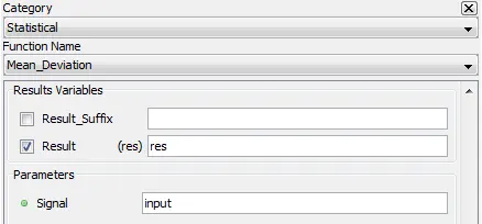
5.4.1.2. Description
Outputs the cummulative distribution function of a signal. The cummulative distribution evaluated at ![]() represents the probability that a random variable following the signal density function takes on a value less than or equal to
represents the probability that a random variable following the signal density function takes on a value less than or equal to ![]() and is given by:
and is given by:
![]()
5.4.1.3. Result Variables and Parameters
Result: Cumulative distribution function
Signal: Input
Nclasses = number of cumulative probability samples evenly distributed
5.4.1.4. Syntax
res=cumprob(input, Nclasses)
5.4.1.5. Characteristics
|
Data type support |
Double Floating point |
5.4.1.6. Example
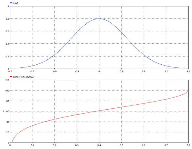
5.4.2. Gaussian Distribution – [gauss]
Outputs a gaussian distribution
5.4.2.1. Category
Statistical
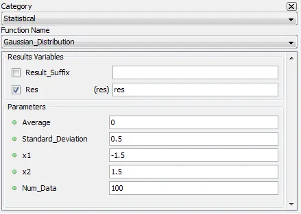
5.4.2.2. Description
Outputs a gaussian distribution of mean “Average”, standard deviation “Standard_Deviation” in the range [x1, x2]. “Num_data” samples evenly distributed over the interval [x1, x2] are generated.
5.4.2.3. Result Variables and Parameters
Result: Gaussian distribution
Average: mean of the Gaussian distribution
Standard_deviation: standard deviation of the Gaussian distribution
x1: lower interval boundary
x2: upper interval boundary
Num_Data= number of samples evenly distributed over [x1, x2] to generate
5.4.2.4. Syntax
res=gauss(Average,Standard_Deviation,x1,x2,Num_Data)
5.4.2.5. Characteristics
|
Data type support |
Double Floating point |
5.4.2.6. Example
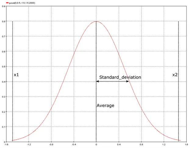
5.4.3. Mean Deviation – [meandev]
Outputs the mean deviation of the input.
5.4.3.1. Category
Statistical
5.4.3.2. Description
Outputs the mean deviation of the input which is given by:
![]()
where ![]() is the mean value of the signal, N the number of samples and
is the mean value of the signal, N the number of samples and ![]() the
the ![]() -th value of the signal
-th value of the signal
5.4.3.3. Result Variables and Parameters
Result: Mean deviation
Signal: Input
5.4.3.4. Syntax
res=meandev(input)
5.4.3.5. Characteristics
|
Data type support |
Double Floating point |
5.4.3.6. Example
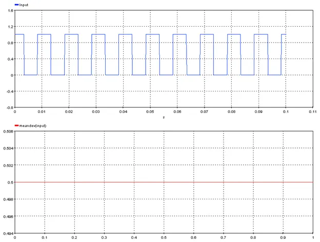
Outputs the p-value of a given signal
5.4.4.1. Category
Statistical

5.4.4.2. Description
Outputs the p-value of a given signal (Signal) for given probability (percentage) were the p-value is defined by the value that has “percentage” chance of being exeeded given the density function defined by the input signal (computed using the cumulative probability of the density function defined by the input signal).
5.4.4.3. Result Variables and Parameters
Result: p-value
Signal: Input
Nclasses = number of samples evenly distributed used to compute the cumulative probability
percentage: percentage at which the p-value must be computed
5.4.4.4. Syntax
res=pvalue(Signal,Nclasses,percentage)
5.4.4.5. Characteristics
|
Data type support |
Double Floating point |
5.4.4.6. Example
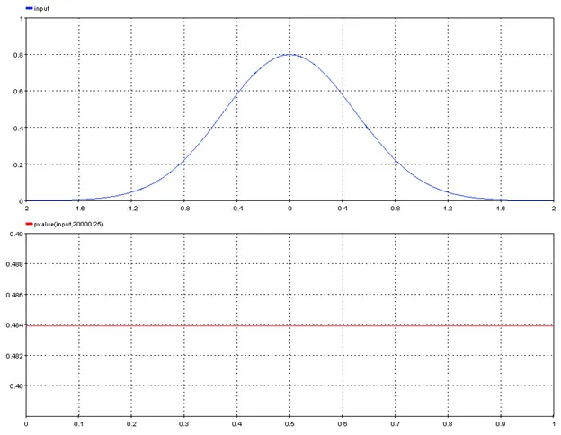
5.4.5. Standard deviation – [stddev]
Outputs the standard deviation of input.
5.4.5.1. Category
Statistical
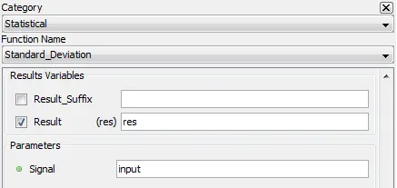
5.4.5.2. Description
Outputs the standard deviation of input.
5.4.5.3. Result Variables and Parameters
Result: Standard deviation
Signal: Input
5.4.5.4. Syntax
res=stddev(input)
5.4.5.5. Characteristics
|
Data type support |
Double Floating point |
5.4.5.6. Example
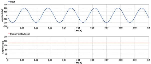
5.4.6. Statistical Frequency – [statfreq]
Outputs the number of values occurences of a signal
5.4.6.1. Category
Statistical
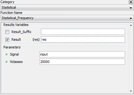
5.4.6.2. Description
Outputs the absolute number of values occurences of a signal. It can be seen as the histogram of the values taken by the inputs where the bin size is given by the difference between the maximum and the minimum value of the signal divided by “Nclasses”.
5.4.6.3. Result Variables and Parameters
Result: Statistical frequency
Signal: Input
Nclasses = number of samples evenly distributed used to compute the statistical frequency
5.4.6.4. Syntax
res= statfreq(Signal,Nclasses)
5.4.6.5. Characteristics
|
Data type support |
Double Floating point |
5.4.6.6. Example
5.5.1. Fast Fourier Transform – [fft]
Outputs the magnitude and the angle for the Fourier series coefficients of selected signal.
5.5.1.1. Category
Harmonic Analysis
5.5.1.2. Description
Outputs the magnitude and the angle for the Fourier series coefficients of the selected signal.
5.5.1.3. Result Variables and Parameters
Magnitude: Magnitude of the Fourier series coefficients at a given frequency.
Phase angle: Angle of the Fourier series coefficients at a given frequency.
Signal: Input
5.5.1.4. Syntax
[m,p]=fft(input)
5.5.1.5. Characteristics
|
Data type support |
Double Floating point |
5.5.1.6. Example
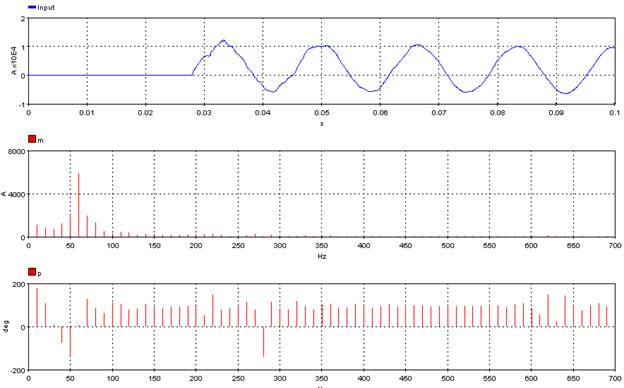
5.5.2. Fundamental Frequency – [ffreq]
Outputs the fundamental frequency of selected signal.
5.5.2.1. Category
Harmonic Analysis
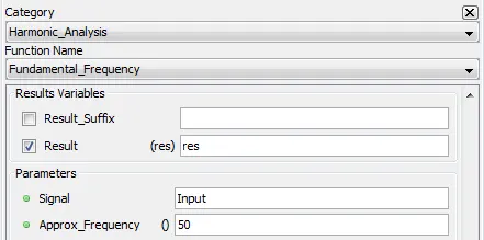
5.5.2.2. Description
Outputs the fundamental frequency of selected signal using least-squares method.
5.5.2.3. Result Variables and Parameters
Result: Fundamental frequency value of the input.
Signal: Input
Approx_Frequency: Search for fundamental frequency using this value as a center point. (optional)
5.5.2.4. Syntax
res=ffreq(input)
res=ffreq(input, approx_freq)
5.5.2.5. Characteristics
|
Data type support |
Double Floating point |
5.5.2.6. Example
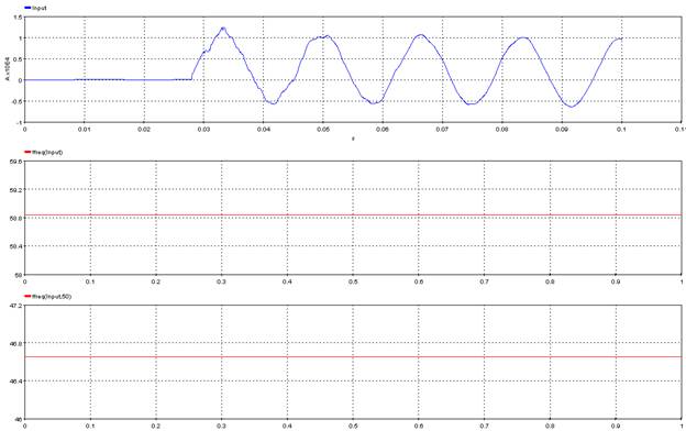
5.5.3. Fundamental Frequency Signal – [ffreqs]
Outputs the fundamental frequency of selected signal evaluated at each data points.
5.5.3.1. Category
Harmonic Analysis
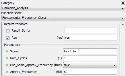
5.5.3.2. Description
Outputs the fundamental frequency of selected signal using an interval around each points.
5.5.3.3. Result Variables and Parameters
Result: Fundamental frequency value at each points of the input signal.
Signal: Input
Num_Cycles: Width factor of the window use to evaluate each fundamentals frequencies. (optional, default=1)
Use_Same_approx_Frequency: Use the same Approx._Frequency for each interval of approximation. If false, use the frequency from the previous interval. (optional, default=true)
Approx_Frequency: Search for fundamental frequency around this value (optional, default=Bloc frequency)
5.5.3.4. Syntax
res=ffreqs(input, num_cycles, use_same_approx_freq, approx_freq)
5.5.3.5. Characteristics
|
Data type support |
Double Floating point |
5.5.3.6. Example
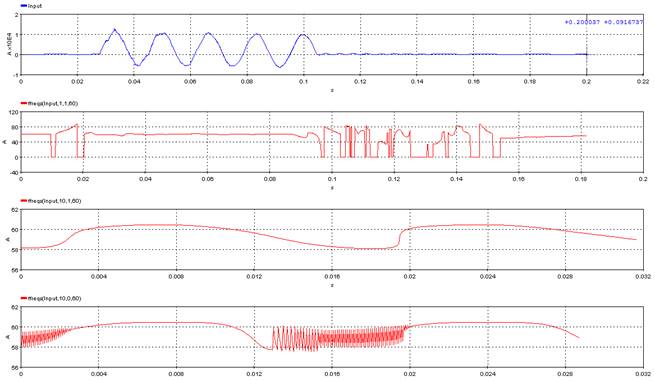
Outputs the module and phase of all selected harmonics over the entire signal.
5.5.4.1. Category
Harmonic Analysis
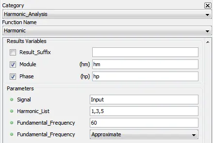
5.5.4.2. Description
Outputs the module and phase of all selected harmonics over the entire signal.
5.5.4.3. Result Variables and Parameters
Module: Module of each selected harmonics.
Phase: Phase of each selected harmonics.
Signal: Input
Harmonic_List: List of harmonic to look at.
Fundamental_Frequency: Value used has the fundamental frequency.
Fundamental_Frequency: Exact: use the provided value. Approximate: search for fundamental frequency around this value.
5.5.4.4. Syntax
[hm,hp]=harm(input, harmonic_list, fundamental_frequency, fundamental_frequency_approx)
5.5.4.5. Characteristics
|
Data type support |
Double Floating point |
5.5.4.6. Example
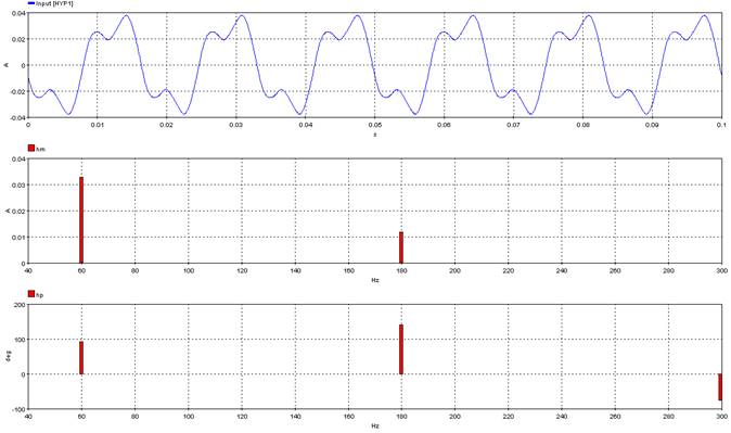
5.5.5. Harmonic Module – [hmod]
Outputs the module of the selected harmonic over time.
5.5.5.1. Category
Harmonic Analysis
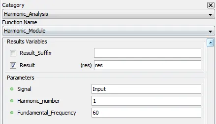
5.5.5.2. Description
Outputs the module of the selected harmonic over time.
5.5.5.3. Result Variables and Parameters
Result: Module of the selected harmonics over time.
Signal: Input
Harmonic_number: The harmonic number.
Fundamental_Frequency: Value used has the fundamental frequency.
5.5.5.4. Syntax
res=hmod(input, harmonic_number, fundamental_frequency)
5.5.5.5. Characteristics
|
Data type support |
Double Floating point |
5.5.5.6. Example
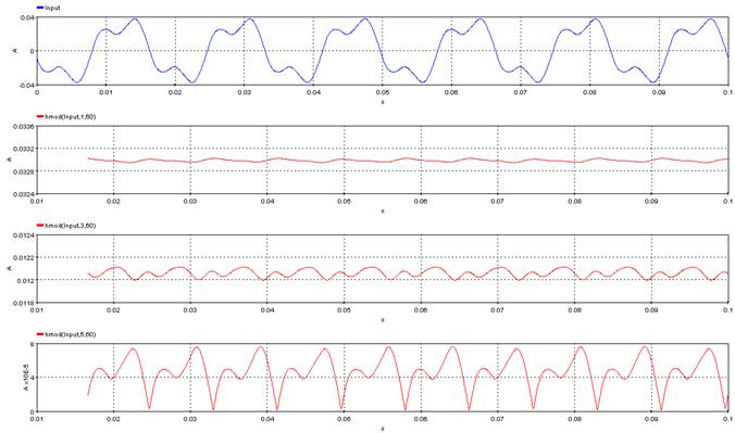
5.5.6. Harmonic Phase – [hpha]
Outputs the module of the selected harmonic over time.
5.5.6.1. Category
Harmonic Analysis
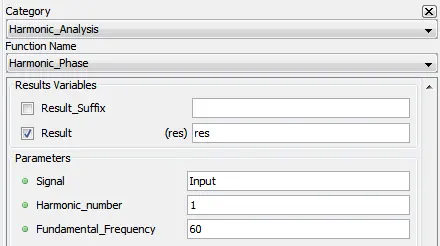
5.5.6.2. Description
Outputs the phase of the selected harmonic over time.
5.5.6.3. Result Variables and Parameters
Result: Phase of the selected harmonics over time.
Signal: Input
Harmonic_number: The harmonic number.
Fundamental_Frequency: Value used has the fundamental frequency.
5.5.6.4. Syntax
res=hpha(input, harmonic_number, fundamental_frequency)
5.5.6.5. Characteristics
|
Data type support |
Double Floating point |
5.5.6.6. Example
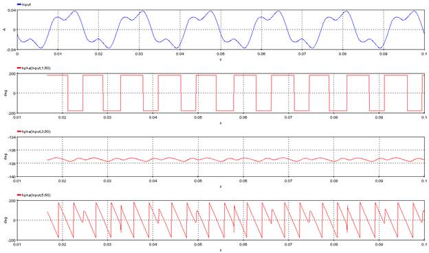
5.5.7. Sequence impedance – [zseq]
Compute the sequence impedance matrix in function of the phase impedance matrix. The input and output are represented by phasors.
5.5.7.1. Category
Harmonic_Analysis
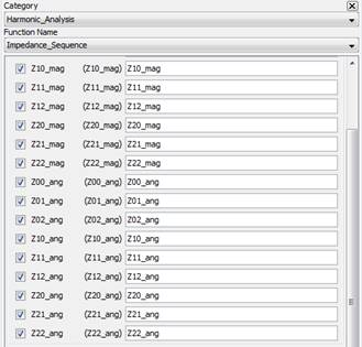
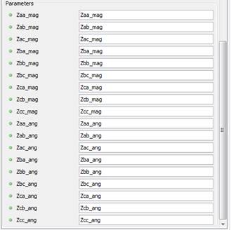
5.5.7.2. Description
Output the sequence impendance matrix in function of an phase impedance matrix. The following equations are used to calculate the impedences:
![]()
![]()
![]()
![]()
![]()
![]()
![]()
![]()
5.5.7.3. Result Variables and Parameters
Results:
Z00_mag : Magnitude of the Z00
Z01_mag : Magnitude of the Z01
Z02_mag : Magnitude of the Z02
Z10_mag : Magnitude of the Z10
Z11_mag : Magnitude of the Z11
Z12_mag : Magnitude of the Z12
Z20_mag : Magnitude of the Z20
Z21_mag : Magnitude of the Z21
Z22_mag : Magnitude of the Z22
Z00_ang : Angle of the Z00 (in degrees)
Z01_ang : Angle of the Z01 (in degrees)
Z02_ang : Angle of the Z02 (in degrees)
Z10_ang : Angle of the Z10 (in degrees)
Z11_ang : Angle of the Z11 (in degrees)
Z12_ang : Angle of the Z12 (in degrees)
Z20_ang : Angle of the Z20 (in degrees)
Z21_ang : Angle of the Z21 (in degrees)
Z22_ang : Angle of the Z22 (in degrees)
Signals:
Zaa_mag : Magnitude of the Zaa
Zab_mag : Magnitude of the Zab
Zac_mag : Magnitude of the Zac
Zba_mag : Magnitude of the Zba (not required)
Zbb_mag : Magnitude of the Zbb
Zbc_mag : Magnitude of the Zbc
Zca_mag : Magnitude of the Zca (not required)
Zcb_mag : Magnitude of the Zcb (not required)
Zca_mag : Magnitude of the Zcc
Zaa_ang : Angle of the Zaa (in degrees)
Zab_ang : Angle of the Zab (in degrees)
Zac_ang : Angle of the Zac (in degrees)
Zba_ang : Angle of the Zba (in degrees) (not required)
Zbb_ang : Angle of the Zbb (in degrees)
Zbc_ang : Angle of the Zbc (in degrees)
Zca_ang : Angle of the Zca (in degrees)
Zcb_ang : Angle of the Zcb (in degrees) (not required)
Zcc_ang : Angle of the Zcc (in degrees) (not required)
5.5.7.4. Syntax
[Z00_mag, Z01_mag, Z02_mag, Z10_mag, Z11_mag, Z12_mag, Z20_mag, Z21_mag, Z22_mag, Z00_ang, Z01_ang, Z02_ang, Z10_ang, Z11_ang, Z12_ang, Z20_ang, Z21_ang, Z22_ang]=zseq( Zaa_mag, Zab_mag, Zac_mag, Zba_mag, Zbb_mag, Zbc_mag, Zca_mag, Zcb_mag, Zcc_mag, Zaa_ang, Zab_ang, Zac_ang, Zba_ang, Zbb_ang, Zbc_ang, Zca_ang, Zcb_ang, Zcc_ang)
5.5.7.5. Characteristics
|
Data type support |
Double Floating point |
5.5.7.6. Example
For this example, a phase impedance matrix is created and the sequence impedance will be computed by zseq function.
This matrix is imported through ScopeView:
![]()
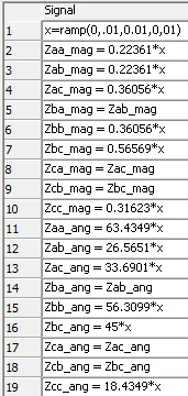
Using the zseq function and putting the result in a table:
![]()
![]()
![]()
Which correspond to this matrix:
![]()
5.5.8. Symmetrical Component Module – [syhmod]
Extract the magnitude of the phasor component from the three input signal.
5.5.8.1. Category
Harmonic Analysis
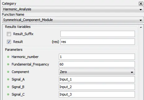
5.5.8.2. Description
Extract the magnitude of the phasor component from the three input signal.
5.5.8.3. Result Variables and Parameters
Result: Module of the phasor component.
Harmonic_number: The harmonic number.
Fundamental_Frequency: Value used has the fundamental frequency.
Signal_A: Input_1
Signal_B: Input_2
Signal_C: Input_3
5.5.8.4. Syntax
res=syhmod(harmonic_number, fundamental_frequency, input_1, input_2, input_3)
5.5.8.5. Characteristics
|
Data type support |
Double Floating point |
5.5.8.6. Example

5.5.9. Symmetrical Component Phase – [sypha]
Extract the phase of the phasor component from the three input signal.
5.5.9.1. Category
Harmonic Analysis

5.5.9.2. Description
Extract the phase of the phasor component from the three input signal.
5.5.9.3. Result Variables and Parameters
Result: Phase of the phasor component.
Harmonic_number: The harmonic number.
Fundamental_Frequency: Value used has the fundamental frequency.
Signal_A: Input_1
Signal_B: Input_2
Signal_C: Input_3
5.5.9.4. Syntax
res=syhpha(harmonic_number, fundamental_frequency, input_1, input_2, input_3)
5.5.9.5. Characteristics
|
Data type support |
Double Floating point |
5.5.9.6. Example
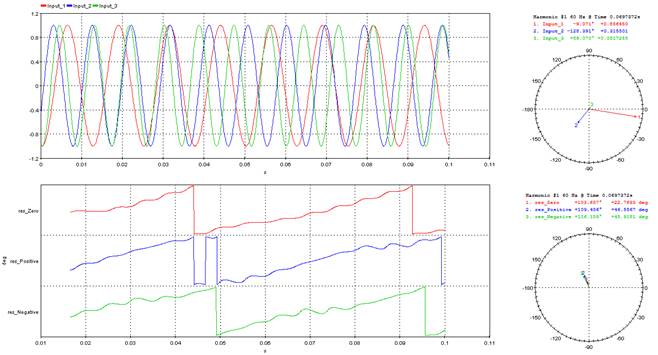
5.5.10. Total Harmonic Distortion – [thd]
Output the total harmonic distortion of the input signal.
5.5.10.1. Category
Harmonic Analysis
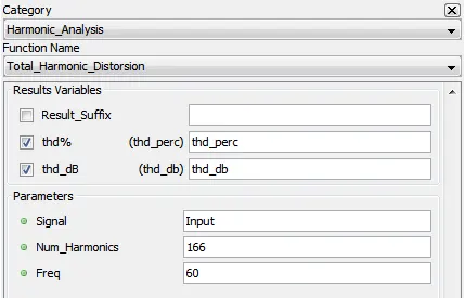
5.5.10.2. Description
Output the total harmonic distortion of the input signal:

![]()
5.5.10.3. Result Variables and Parameters
Thd%: Total harmonic distortion value in percent.
Thd_db: Total harmonic distortion value in db.
Signal: Input
Num_Harmonics: Number of harmonic use to calculate the THD.
Freq: Value used has the fundamental frequency.
5.5.10.4. Syntax
[thd_perc,thd_db] = thd(input,num_harmonics,freq)
5.5.10.5. Characteristics
|
Data type support |
Double Floating point |
5.5.10.6. Example
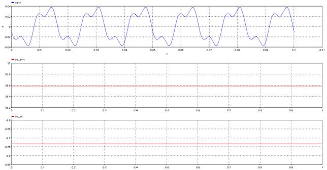
5.6.1. Linear Interpolation – [interpl]
Outputs the input signal’s linear interpolation
5.6.1.1. Category
Miscellaneous
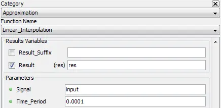
5.6.1.2. Description
Outputs the input signal linear interpolation with a given sampling time (Time_Period)
5.6.1.3. Result Variables and Parameters
Signal: input signal
Time_Period: output sampling time
5.6.1.4. Syntax
res= interpl(input,0.0001)
5.6.1.5. Characteristics
|
Data type support |
Double Floating point |
5.6.1.6. Example
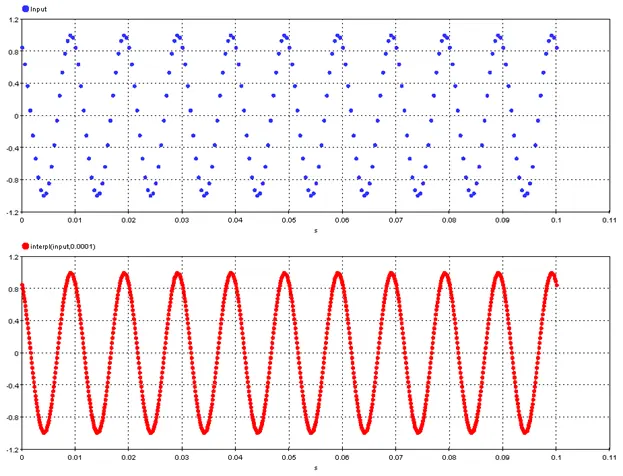
5.7.1. Type of windows for the following functions:
5.7.1.1. Rectangular
A rectangular window will have the signals value inside the window and zero outside the window.
5.7.1.2. Hanning
The Hann window is defined by :
![]()
5.7.1.3. Hamming
The Hamming window is defined by :
![]()
![]()
5.7.1.4. Blackman
The Blackman window is defined by :
![]()
![]()
5.7.2. Cross Spectral Density – [crospec]
Outputs the cross-spectral density of two signals.
5.7.2.1. Category
Spectral analysis
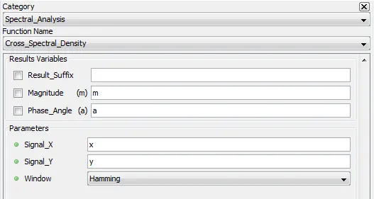
5.7.2.2. Description
Outputs the cross-spectral density by doing a Fast fourier transform on both signals and returning cross-spectral densigy.
5.7.2.3. Result Variables and Parameters
Magnitude (m): Cross-spectral density magnitude
Phase_Angle (a): Cross-spectral density phase
Signal_X: First signal to use for the cross-spectral density
Signal_Y: Second signal to use for the cross-spectral density
Window: Type of windowing applied to the analyzed samples. Refer to the beginning of Spectral analysis category to have a short description. [0: Rectangular,1: Hanning, 2: Hamming, 3: Blackman]
5.7.2.4. Syntax
[m,a]=crospec(x,y,2)
5.7.2.5. Characteristics
|
Data type support |
Double Floating point |
5.7.2.6. Example
Here are the results of the cross-spectral density of:
x=sin(pi*2*15*t)
y=sin(pi*2*15*t+90*360/(pi*2)) + sin( pi*2*28*t+90*360/(pi*2))
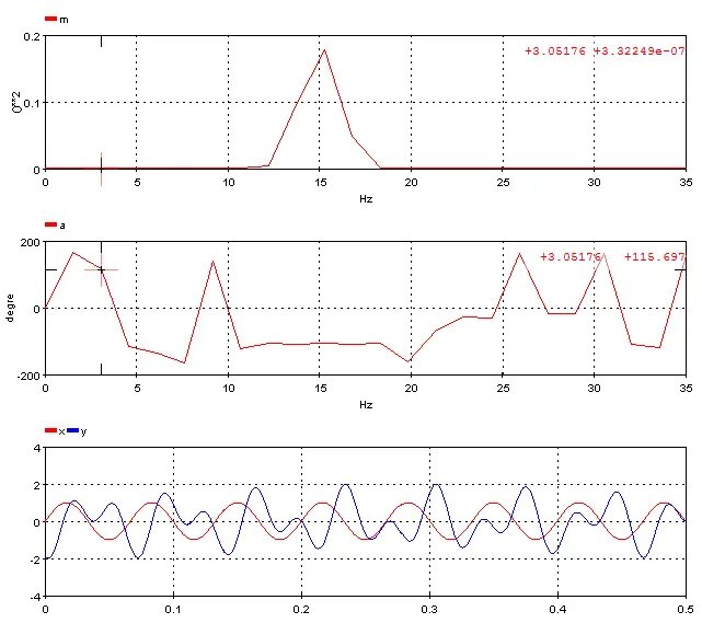
5.7.3. Frequency Response – [repfreq]
Outputs the transfer function by comparing two Fast Fourier Transformation signal.
5.7.3.1. Category
Spectral analysis
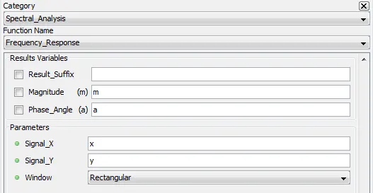
5.7.3.2. Description
Outputs the magnitudes and phases of the transfer function. The analysis is based on the Fast Fourier Transform of inputs signals.
5.7.3.3. Result Variables and Parameters
Magnitude (m): Frequency response magnitude
Phase_Angle (a): Frequency response phase
Signal_X: First signal to use for the frequency response analysis
Signal_Y: Second signal to use for the frequency response analysis
Window: Type of windowing applied to the analyzed samples. Refer to the beginning of Spectral analysis category to have a short description. [0: Rectangular,1: Hanning, 2: Hamming, 3: Blackman]
5.7.3.4. Syntax
res= statfreq(Signal,Nclasses)
5.7.3.5. Characteristics
|
Data type support |
Double Floating point |
5.7.3.6. Example
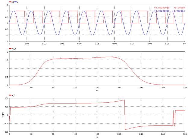
5.7.4. Spectral Density – [densp]
Outputs the spectral density of a signal.
5.7.4.1. Category
Spectral analysis
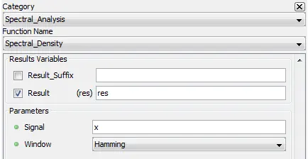
5.7.4.2. Description
Output the spectral density plot in function of an input signal. Windowing is used for sampling
5.7.4.3. Result Variables and Parameters
Result: Spectral density result
Signal: Input signal
Window: Type of windowing applied to the analyzed samples. Refer to the beginning of Spectral analysis category to have a short description. [0: Rectangular,1: Hanning, 2: Hamming, 3: Blackman]
5.7.4.4. Syntax
res=densp(y,2)
5.7.4.5. Characteristics
|
Data type support |
Double Floating point |
5.7.4.6. Example
Spectral analysis of a 15 Hz and 28 Hz sinusoidal sum.
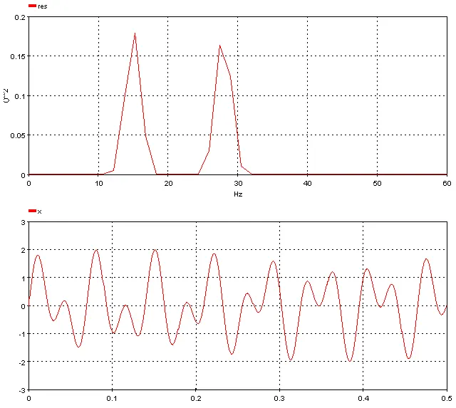
5.8.1. Overshoot time – [sidseuil ]
Computes the period of time during which a threshold value is reached in a signal.
5.8.1.1. Category
SI5
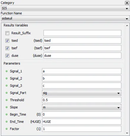
5.8.1.2. Description
The function compute the period of time and different results related to the overshoot time during which a threshold value is reached in a signal, either on a rising or a falling edge. The function computes the beginning and ending time and duration of the threshold condition.
To perform the analysis, a new signal is generated with the three signals specified as input parameters and following the type of threshold specified.
- Rise (m) : the resulting signal is the maximum of the three signals.
- Fall (d): the resulting signal is the minimum of the three signals.
When samples do not belong to the signal part specified, values are replaced 0.0.
The user must specify three input signals. However, if only one signal is to be used, then the same name should be given to all three signals. When only one signal is processed, the maximum and minimum samples will result in one identical signal. Similarly, if two signals are to be processed, the third signal to be used can be identical to one of the first two.
5.8.1.3. Result Variables and Parameters
tsed: From the starting time of the analysis, course of the generated signal to find the time at which the threshold value is reached based on the type of threshold specified. The time is returned in milliseconds [ms] and is relative to time 0.
tsef: From the ending time of the analysis, course of the generated signal towards the beginning to find the time at which the threshold value is reached based on the type of threshold specified. The time is returned in milliseconds [ms] and is relative to time 0.
duse: Difference between tsef and tsed in milliseconds [ms]. This result represents the period of time during which the threshold value is reached.
Signal_1: First signal to analyze.
Signal_2: Second signal to analyze.
Signal_3: Third signal to analyze.
Signal_Part: Part of the signal on which the analysis is done (neg, pos, sig, abs). Here are the definitions for the four distinct parts of a signal:
- Neg : Only the negative values of the input signal are used for the calculations. The other values are considered to be null.
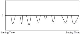
- Pos : Only the positive values of the input signal are used for the calculations. The other values are considered to be null.
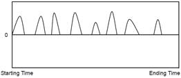
- Sig : The original input signal is used for the calculations.
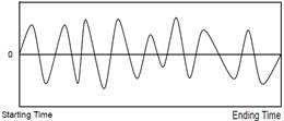
- Abs : The calculations are done on the absolute value of the input signal.
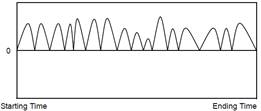
Threshold: Value of threshold to be reached on the specified part of the signal.
Slope: Type of threshold to reach: the threshold value can be reached on a rise (m) or a fall (d).
- Rise (m): On the resulting signal, the threshold is considered to be reached when the first sample of the analyzed signal exceeds the specified threshold (tsed). From the ending time of the analysis, the threshold is considered to end when the first sample of the analyzed signal exceeds the specified threshold (tsef).
- Fall (d): On the resulting signal, the threshold is considered to be reached when the first sample is smaller than the specified threshold (tsed). From the ending time of the analysis, the threshold is considered to end when the first sample of the analyzed signal is smaller than the specified threshold (tsef).
Begin_time: Time at which the analysis of a signal must start. This time is expressed in milliseconds [ms]. This value must be greater than 0 and lower than the size of the acquisition buffer. The default value is 0.
End_time: Time at which the analysis of a signal must end. This time is expressed in milliseconds [ms]. The value of this time must be larger than the specified begin_time and smaller than the duration of the test. Use the “HUGE” value to specify the end of the test. The default value is HUGE.
Factor: Multiplying factor for the results generated by the function. The default value of the multiplying factor is 1.0 and has no effect on the results. The multiplying factor applies only to the tsed and tsef results.It does not apply to the duse result.
5.8.1.4. Syntax
[tsed, tsef, duse] = sidseuil(sig1, sig2, sig3, "sig", threshold, "m", 0, HUGE, factor)
5.8.1.5. Characteristics
|
Data type support |
Double Floating point |
5.8.1.6. Example
Sidseuil function on a rise:
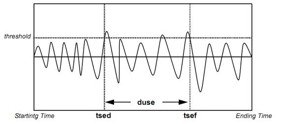
Sidseuil function on a fall:
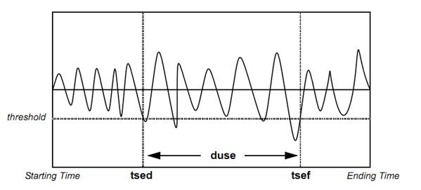
The next figure shows the different limit cases of the Sidseuil function.
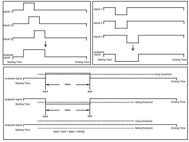
5.8.2. Fundamental Frequency – [sifreq]
Compute the exact fundamental frequency of a signal.
5.8.2.1. Category
SI5
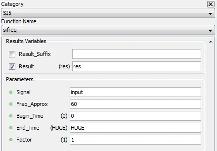
5.8.2.2. Description
Compute the fundamental frequency of the input signal in Hertz [Hz] using an approximate fundamental frequency and using the Brent method
5.8.2.3. Result Variables and Parameters
Result: Fundamental frequency [Hz]. If the function returns zero as a result, this means that the fundamental frequency was not found, probably because the deviation from the approximate fundamental frequency provided is too large.
Signal: Input signal to perform calculation
Freq_Approx: Approximate and initial fundamental frequency in Hz.
Begin_time: Time at which the analysis of a signal must start. This time is expressed in milliseconds [ms]. This value must be greater than 0 and lower than the size of the acquisition buffer. The default value is 0.
End_time: Time at which the analysis of a signal must end. This time is expressed in milliseconds [ms]. The value of this time must be larger than the specified begin_time and smaller than the duration of the test. Use the “HUGE” value to specify the end of the test. The default value is HUGE.
Factor: Multiplying factor for the results generated by the function. The default value of the multiplying factor is 1.0 and has no effect on the results.
5.8.2.4. Syntax
res = sifreq(input, 60, 0, HUGE, 1)
5.8.2.5. Characteristics
|
Data type support |
Double Floating point |
5.8.2.6. Example
5.8.3. Absolute Maximum – [simax1]
Computes the absolute or algebraic maximum on a specific part of a signal.
5.8.3.1. Category
SI5
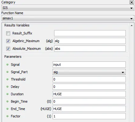
5.8.3.2. Description
This function allows to compute the absolute or algebraic maximum on a specific part of a signal. The zone on which the analysis is performed can be specify using time, or using or a threshold condition.
5.8.3.3. Result Variables and Parameters
Algebraic Maximum: Maximum of the input signal multiplied by the factor.
An algebraic or absolute result on an absolute or positive part of a signal does not affect the result. Similarly, the algebraic result on the negative part of a signal is negative, unless the time interval found for the analysis is null.
Absolute Maximum: Absolute maximum of the input signal multiplied by the factor.
Signal: Input signal to perform calculation
Signal_Part: Part of the signal on which the analysis is done (neg, pos, sig, abs). Here are the definitions for the four distinct parts of a signal:
- Neg : Only the negative values of the input signal are used for the calculations. The other values are considered to be null.
- Pos : Only the positive values of the input signal are used for the calculations. The other values are considered to be null.
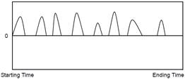
- Sig : The original input signal is used for the calculations.
- Abs : The calculations are done on the absolute value of the input signal.
Threshold: The threshold, delay, and duration parameters restrict the limits of an analysis. The threshold is the value to reach to start the analysis from the begin_time. If the threshold is positive, the threshold will be reached when the value of the sample is greater than that of the threshold. If the threshold is negative, the threshold will be reached when the value of the sample is smaller than that of the threshold. A null threshold sets the threshold equal to the starting time.
The threshold value must be compatible with the signal part specified. If the positive part of a signal is specified with a negative threshold, this threshold will never be reached.
Delay: When the threshold time is determined, a delay is added to it. The new starting time of the analysis is thus equal to the time taken to reach the threshold plus the delay. The delay is specified in milliseconds [ms].
Duration: The duration parameter serves to determine the ending time of the analysis. This ending time will be equal to the new starting time with the delay plus the specified duration. It is possible to specify HUGE as duration indicating that the ending time will be the end of the analyzed signal. This duration is specified in milliseconds [ms].
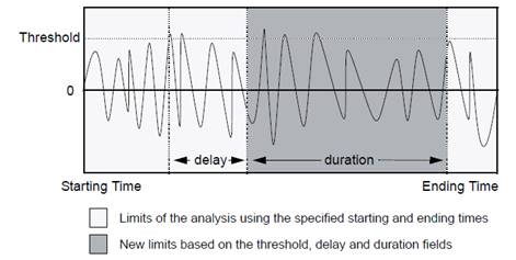
Begin_time: Time at which the analysis of a signal must start. This time is expressed in milliseconds [ms]. This value must be greater than 0 and lower than the size of the acquisition buffer. The default value is 0.
End_time: Time at which the analysis of a signal must end. This time is expressed in milliseconds [ms]. The value of this time must be larger than the specified begin_time and smaller than the duration of the test. Use the “HUGE” value to specify the end of the test. The default value is HUGE.
Factor: Multiplying factor for the results generated by the function. The default value of the multiplying factor is 1.0 and has no effect on the results.
5.8.3.4. Syntax
[alg, abs] = simax1(input, "sig", 0, 0, HUGE, 0, HUGE,1)
5.8.3.5. Characteristics
|
Data type support |
Double Floating point |
5.8.3.6. Example
The following figure shows absolute and algebraic maximum for a sine wave signal.
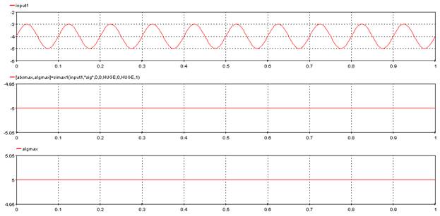
The following diagram shows the different results computed by this function.
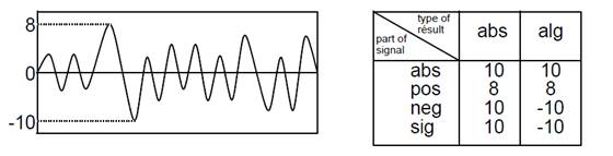
5.8.4. Absolute Maximum – [simax2]
Computes the absolute or algebraic maximum of a signal resulting from a mathematical operation between two signals.
5.8.4.1. Category
SI5
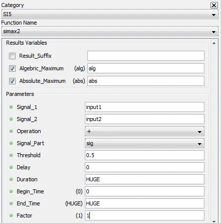
5.8.4.2. Description
This function allows to compute the absolute or algebraic maximum of a signal, or of a part of it, resulting from a mathematical operation between two signals. The zone on which the analysis is performed can be specify using time, or using or a threshold condition.
5.8.4.3. Result Variables and Parameters
Algebraic Maximum: Maximum of the resulting signal multiplied by the factor.
An algebraic or absolute result on an absolute or positive part of a signal does not affect the result. Similarly, the algebraic result on the negative part of a signal is negative, unless the time interval found for the analysis is null.
Absolute Maximum: Absolute maximum of the resulting signal multiplied by the factor.
Signal 1: First input signal to perform the mathematical operation
Signal 2: Second input signal to perform the mathematical operation
Operation: Operation to execute between the two signals to analyze (+, - , *, /)
Signal_Part: Part of the signal on which the analysis is done (neg, pos, sig, abs). Here are the definitions for the four distinct parts of a signal:
- Neg : Only the negative values of the input signal are used for the calculations. The other values are considered to be null.
- Pos : Only the positive values of the input signal are used for the calculations. The other values are considered to be null.
- Sig : The original input signal is used for the calculations.
- Abs : The calculations are done on the absolute value of the input signal.
Threshold: The threshold, delay, and duration parameters restrict the limits of an analysis. The threshold is the value to reach to start the analysis from the begin_time. If the threshold is positive, the threshold will be reached when the value of the sample is greater than that of the threshold. If the threshold is negative, the threshold will be reached when the value of the sample is smaller than that of the threshold. A null threshold sets the threshold equal to the starting time.
The threshold value must be compatible with the signal part specified. If the positive part of a signal is specified with a negative threshold, this threshold will never be reached.
Delay: When the threshold time is determined, a delay is added to it. The new starting time of the analysis is thus equal to the time taken to reach the threshold plus the delay. The delay is specified in milliseconds [ms].
Duration: The duration parameter serves to determine the ending time of the analysis. This ending time will be equal to the new starting time with the delay plus the specified duration. It is possible to specify HUGE as duration indicating that the ending time will be the end of the analyzed signal. This duration is specified in milliseconds [ms].
- 
Begin_time: Time at which the analysis of a signal must start. This time is expressed in milliseconds [ms]. This value must be greater than 0 and lower than the size of the acquisition buffer. The default value is 0.
End_time: Time at which the analysis of a signal must end. This time is expressed in milliseconds [ms]. The value of this time must be larger than the specified begin_time and smaller than the duration of the test. Use the “HUGE” value to specify the end of the test. The default value is HUGE.
Factor: Multiplying factor for the results generated by the function. The default value of the multiplying factor is 1.0 and has no effect on the results.
5.8.4.4. Syntax
[alg_max, abs_max] = simax2(input1, input2, "+", "sig", 0.5, 0, HUGE, 0, HUGE, 1)
5.8.4.5. Characteristics
|
Data type support |
Double Floating point |
5.8.4.6. Example
The following figure shows absolute and algebraic maximum for the sum of sine wave signal and a constant value.
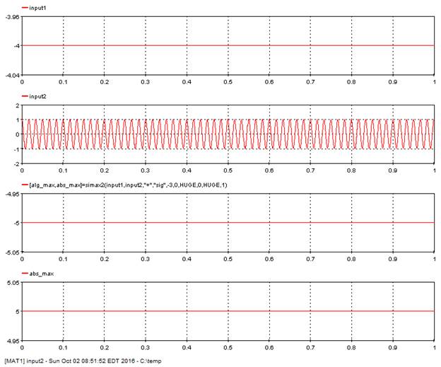
The following diagram shows the different results computed by this function.
5.8.5. Phase Maximum – [simax3]
Computes the absolute and algebraic maximum on a specific part of a signal of a phase to phase or a phase to neutral voltage or a current.
5.8.5.1. Category
SI5
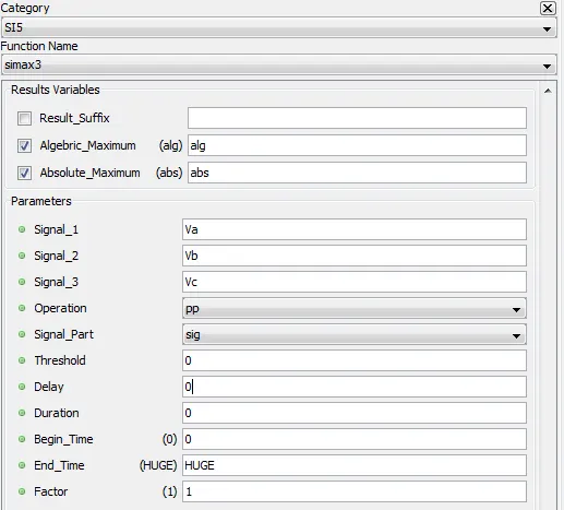
5.8.5.2. Description
The function allows to compute the absolute and algebraic maximum on a specific part of a signal of a phase to phase or a phase to neutral voltage or a current.
5.8.5.3. Result Variables and Parameters
Algebraic Maximum: Maximum of the resulting signal multiplied by the factor.
An algebraic or absolute result on an absolute or positive part of a signal does not affect the result. Similarly, the algebraic result on the negative part of a signal is negative, unless the time interval found for the analysis is null.
Absolute Maximum: Absolute maximum of the resulting signal multiplied by the factor.
Signal_1: input signal (phase a).
Signal_2: input signal (phase b).
Signal_3: input signal (phase c).
For simax3, the three signals are kept to the end. It is as if simax1 were applied to the three analyzed signals and the result returned were the maximum of the three maximums identified.
Operation: Operation to execute between the three signals: phase to phase voltage (pp) or phase to neutral (pt). In the case of phase to neutral, the three original signals are considered. For the phase to phase voltages, the difference signals (1 - 2), (2 - 3) and (3 - 1) are considered.
When phase to phase operation is used, three new signals R1, R2 and R3 are internally generated to perform calculation. R1 = Signal_1 – Signal_2, R2 = Signal_2 – Signal_3, R3 = Signal_3 – Signal_1.
Signal_Part: Part of the signal on which the analysis is done (neg, pos, sig, abs). Here are the definitions for the four distinct parts of a signal:
- Neg : Only the negative values of the input signal are used for the calculations. The other values are considered to be null.
- Pos : Only the positive values of the input signal are used for the calculations. The other values are considered to be null.
- Sig : The original input signal is used for the calculations.
- Abs : The calculations are done on the absolute value of the input signal.
Threshold: The threshold, delay, and duration parameters restrict the limits of an analysis. The threshold is the value to reach to start the analysis from the begin_time. If the threshold is positive, the threshold will be reached when the value of the sample is greater than that of the threshold. If the threshold is negative, the threshold will be reached when the value of the sample is smaller than that of the threshold. A null threshold sets the threshold equal to the starting time.
The threshold value must be compatible with the signal part specified. If the positive part of a signal is specified with a negative threshold, this threshold will never be reached.
Delay: When the threshold time is determined, a delay is added to it. The new starting time of the analysis is thus equal to the time taken to reach the threshold plus the delay. The delay is specified in milliseconds [ms].
Duration: The duration parameter serves to determine the ending time of the analysis. This ending time will be equal to the new starting time with the delay plus the specified duration. It is possible to specify HUGE as duration indicating that the ending time will be the end of the analyzed signal. This duration is specified in milliseconds [ms].
-
Begin_time: Time at which the analysis of a signal must start. This time is expressed in milliseconds [ms]. This value must be greater than 0 and lower than the size of the acquisition buffer. The default value is 0.
End_time: Time at which the analysis of a signal must end. This time is expressed in milliseconds [ms]. The value of this time must be larger than the specified begin_time and smaller than the duration of the test. Use the “HUGE” value to specify the end of the test. The default value is HUGE.
Factor: Multiplying factor for the results generated by the function. The default value of the multiplying factor is 1.0 and has no effect on the results.
5.8.5.4. Syntax
[alg_max, abs_max] = simax3(Va, Vb, Vc, "pp", "sig", 0, 0, 0, 0, HUGE, 1)
5.8.5.5. Characteristics
|
Data type support |
Double Floating point |
5.8.5.6. Example
The following figure shows absolute and algebraic maximum for three phase voltages.
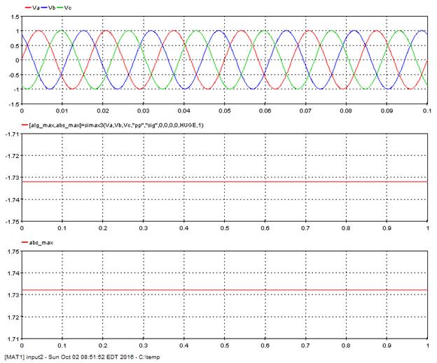
The following diagram shows the different results computed by this function.
Computes the harmonics of a signal.
5.8.6.1. Category
SI5
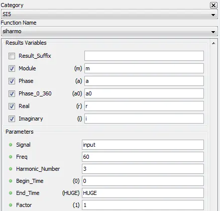
5.8.6.2. Description
The function allows to compute the harmonics of a signal using the exact fundamental frequency. This function computes module (amplitude), angle (phase) and the real and imaginary parts of the harmonics.
5.8.6.3. Result Variables and Parameters
Module (m): Module (or amplitude) for the symmetric components of a harmonic.
Phase (a): Angle a (or phase) of the symmetric component sequence, between -180 and 180 degrees [°].
Phase (a0): Angle of the symmetric component sequence, found between 0 and 360 degrees [°].
Real (r): Real part r of the required symmetric component sequence (m * cos(a)).
Imaginary (i): Imaginary part i of the required symmetric component sequence (m * sin(a)).
Signal: Input signal to perform analysis
Freq: Fundamental frequency of the signal in Hertz [Hz], normally computed with the sifreq function.
Harmonic number: Number of harmonic to compute.
· 0: DC;
· 1: Fundamental;
· 2: 2nd harmonic;
· n: nth harmonic (max. 30).
Begin_time: Time at which the analysis of a signal must start. This time is expressed in milliseconds [ms]. This value must be greater than 0 and lower than the size of the acquisition buffer. The default value is 0.
End_time: Time at which the analysis of a signal must end. This time is expressed in milliseconds [ms]. The value of this time must be larger than the specified begin_time and smaller than the duration of the test. Use the “HUGE” value to specify the end of the test. The default value is HUGE.
Note : The begin time and end time specified for the calculation of the harmonics must be identical to those used in the sifreq sequences which served to compute the fundamental frequency.
Factor: Multiplying factor for the results generated by the function. The default value of the multiplying factor is 1.0 and has no effect on the results. The module is multiplied by the absolute value of thefactor. Hence, the phase is modified if the multiplying factor is negative. In this case, 180 degrees are added to the phase.
5.8.6.4. Syntax
[m, a, a0, r, i] = siharmo(input, freq,n,begin,end,factor)
5.8.6.5. Characteristics
|
Data type support |
Double Floating point |
5.8.6.6. Example
In the following example, the harmonics function compute the third harmonic components of a signal. Module and angle are shown.
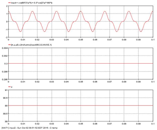
5.8.7. Harmonic Maximum – [simxhart]
Computes the maximum of the amplitudes of a given harmonic.
5.8.7.1. Category
SI5
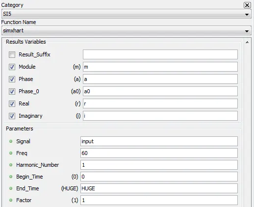
5.8.7.2. Description
The function allows to compute the maximum of the amplitudes of a given harmonic in a moving window over a signal. This window is equal to the length of a cycle with respect to the fundamental frequency. This function computes module (amplitude) and angle (phase) for the symmetric components and its real and imaginary components.
If the number of samples to establish the length of a cycle is greater than the number of samples found between the starting and ending times of the sequence, then the length of the window used is equal to the number of samples between the starting and ending times (in other words ending time starting-time).
5.8.7.3. Result Variables and Parameters
Module (m): Maximum of module (or amplitude) for the symmetric components of a harmonic. It is computed for each window moving over the signal, multiplied by the absolute value of the factor.
Phase (a): Angle a (or phase) of the symmetric component sequence associated with the maximum module found. Value is between -180 and 180 degrees [°].
Since the module is multiplied by the absolute value of the factor, the phase is modified if the multiplying factor is negative. In this case, 180 degrees are added to the phase.
Phase (a0): Angle a0 (or phase) of the symmetric component sequence associated with the maximum module found. Value is between 0 and 360 degrees [°].
Real (r): Real part r of the required symmetric component sequence (m * cos(a)).
Imaginary (i): Imaginary part i of the required symmetric component sequence (m * sin(a)).
Signal: Input signal to perform analysis
Freq: Fundamental frequency of the signal in Hertz [Hz], normally compute with the sifreq function. This fundamental frequency in hertz serves to establish the length of time the window moves over the analyzed signal. In fact, this window is equal to one cycle (in number of samples). lfen = rate/ freq [samples].
Harmonic number: Number of harmonic to compute.
· 0: DC;
· 1: Fundamental;
· 2: 2nd harmonic;
· n: nth harmonic (max. 30).
Begin_time: Time at which the analysis of a signal must start. This time is expressed in milliseconds [ms]. This value must be greater than 0 and lower than the size of the acquisition buffer. The default value is 0.
End_time: Time at which the analysis of a signal must end. This time is expressed in milliseconds [ms]. The value of this time must be larger than the specified begin_time and smaller than the duration of the test. Use the “HUGE” value to specify the end of the test. The default value is HUGE.
Note : The begin_time and end_time specified for the calculation of the harmonics must be the same as those used in the sifreq sequences used to compute the fundamental frequency.
Factor: Multiplying factor for the results generated by the function. The default value of the multiplying factor is 1.0 and has no effect on the results.
5.8.7.4. Syntax
[m, a, a0, r, i] = simxhart( input, 60, 1, 0, HUGE, 1)
5.8.7.5. Characteristics
|
Data type support |
Double Floating point |
5.8.7.6. Example
In the following example, the function compute amplitude maximum of the third harmonic components of a signal.
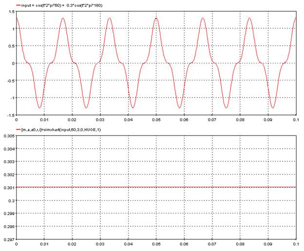
The following diagram shows a window moving over a signal. The method used to compute the length of the window is also described.
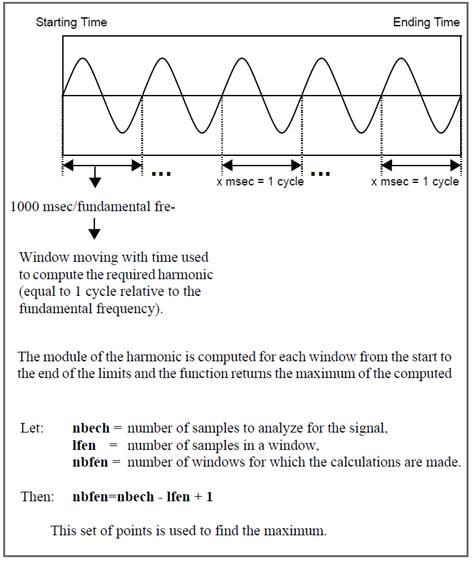
5.8.8. Integral maximum – [simxsom1]
Computes the absolute maximum of an integral, a mean or a RMS value on a specific part of a signal and in a window moving.
5.8.8.1. Category
SI5
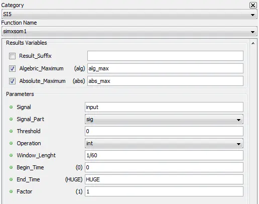
5.8.8.2. Description
The function allows to compute the absolute maximum of an integral, a mean or a RMS value on a specific part of a signal and in a window moving over the input signal.
5.8.8.3. Result Variables and Parameters
Algebraic Maximum: Maximum of the input signal, multiplied by the factor.
Absolute Maximum: Absolute maximum of the input signal, multiplied by the factor.
Signal: Input signal to perform analysis
Signal_Part: Part of the signal on which the analysis is done (neg, pos, sig, abs). Here are the definitions for the four distinct parts of a signal:
- Neg : Only the negative values of the input signal are used for the calculations. The other values are considered to be null.
- Pos : Only the positive values of the input signal are used for the calculations. The other values are considered to be null.
- Sig : The original input signal is used for the calculations.
- Abs : The calculations are done on the absolute value of the input signal.
Threshold: Threshold to reach in order to start analyzing the signals. This threshold value must be positive since the absolute value of the sample is compared to it. The samples which do not exceed this threshold are considered as null. If this threshold is null, all the samples are automatically considered.
Operation: Operation to execute on the signal in a window moving over it (int, moy, rms). The maximum of the integrals, means or RMS values are kept.
· int: integral,
· moy: mean,
· rms: rms value.
Window_Length: Time in seconds [s] during which the window moves over the analyzed signal. This time in seconds is reduced to the time of the analysis (end_time – begin_time), if the window time specified is longer than the duration considered for the signal. This window time cannot be null.
Begin_time: Time at which the analysis of a signal must start. This time is expressed in milliseconds [ms]. This value must be greater than 0 and lower than the size of the acquisition buffer. The default value is 0.
End_time: Time at which the analysis of a signal must end. This time is expressed in milliseconds [ms]. The value of this time must be larger than the specified begin_time and smaller than the duration of the test. Use the “HUGE” value to specify the end of the test. The default value is HUGE.
Factor: Multiplying factor for the results generated by the function. The default value of the multiplying factor is 1.0 and has no effect on the results.
5.8.8.4. Syntax
[alg_max, abs_max] = simxsom1( input, "sig", 0, "int", 1/60, 0, HUGE, 1 )
5.8.8.5. Characteristics
|
Data type support |
Double Floating point |
5.8.8.6. Example
In the following example, the function compute the absolute maximum of the integral of the sine wave over a moving window.
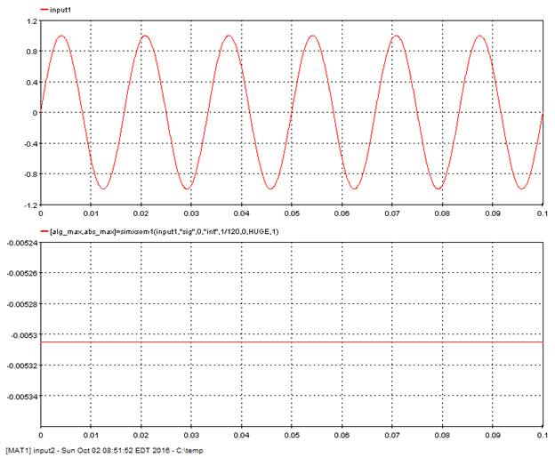
The following diagram shows the window moving over a signal based on the time specified for the window.
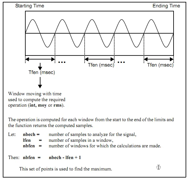
5.8.9. Integral maximum – [simxsom2]
Computes the absolute maximum of an integral, a mean or a RMS value in a window moving over a signal resulting from a mathematical operation.
5.8.9.1. Category
SI5
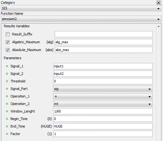
5.8.9.2. Description
The function allows to computes the absolute maximum of an integral, a mean or a RMS value in a window moving over a signal resulting from a mathematical operation between specific parts of two initial signals. A reject threshold can be applied to the first signal before the mathematical operation, in other words the reject of the signal samples not reaching this threshold.
5.8.9.3. Result Variables and Parameters
Algebraic Maximum: Maximum of the input signal, multiplied by the factor.
Absolute Maximum: Absolute maximum of the input signal, multiplied by the factor.
Signal 1: First input signal to perform analysis
Signal 2: Second input signal to perform analysis
Threshold: Threshold to reach on the first signal to keep the sample. This threshold value must be positive since the absolute value of the sample is compared to it. The samples which do not exceed this threshold are considered as null. If this threshold is null, all the samples are automatically considered.
Signal_Part: Part of the signal on which the analysis is done (neg, pos, sig, abs). Here are the definitions for the four distinct parts of a signal:
- Neg : Only the negative values of the input signal are used for the calculations. The other values are considered to be null.
- Pos : Only the positive values of the input signal are used for the calculations. The other values are considered to be null.
- Sig : The original input signal is used for the calculations.
- Abs : The calculations are done on the absolute value of the input signal.
Operation_1: Mathematical operation to execute between the two input signals (+,-,*,/).
Operation_2: Operation to execute on the signal resulting from the mathematical operation in a window moving over it (int, moy, rms). The maximums of the integrals, means or rms values are kept.
· int: integral
· moy: mean
· rms: rms value
Window_Length: Time in seconds [s] during which the window moves over the analyzed signal. This time is reduced to the time of the analysis (ending time - starting time) if the window time specified is longer than the duration considered for the signal. This window time cannot be null.
Begin_time: Time at which the analysis of a signal must start. This time is expressed in milliseconds [ms]. This value must be greater than 0 and lower than the size of the acquisition buffer. The default value is 0.
End_time: Time at which the analysis of a signal must end. This time is expressed in milliseconds [ms]. The value of this time must be larger than the specified begin_time and smaller than the duration of the test. Use the “HUGE” value to specify the end of the test. The default value is HUGE.
Factor: Multiplying factor for the results generated by the function. The default value of the multiplying factor is 1.0 and has no effect on the results.
5.8.9.4. Syntax
[alg_max, abs_max] = simxsom1( input, "sig", 0, "int", 1/60, 0, HUGE, 1 )
5.8.9.5. Characteristics
|
Data type support |
Double Floating point |
5.8.9.6. Example
In the following example, the function compute the absolute maximum of the integral of the sum of two sine waves.
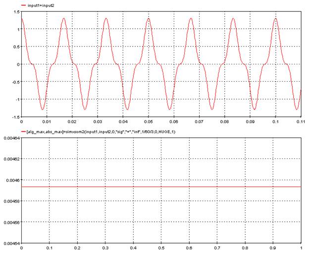
The following diagram shows the window moving over a signal based on the time specified for the window.
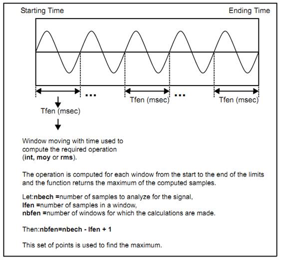
5.8.10. Dynamic Response – [sidyn2]
Computes the dynamic response of a control signal following a disturbance.
5.8.10.1. Category
SI5
5.8.10.2. Description
The function computes the dynamic response of a control system after a disturbance. This function allows to compute mean, minimum and maximum values and stabilization times.
Note : The order of operations of this function is not as important as for other functions, but it is useful to know.
1- Course of the signal from reference Ref_Time1 to reference Ref_Time2 to find the minimum and maximum of the disturbance.
2- Calculation of the mean on the Interval (moyd) first milliseconds, of the mean on the interval (moyf) last milliseconds and of the mean on the Interval (moyp) milliseconds preceding reference Ref_Time2. These values are returned as the moyd, moyf and moyp results.
3- Calculation of time taken to reach the different threshold values for the stabilization times.
5.8.10.3. Result Variables and Parameters
maxp: Maximum value of the input signal between first and second reference times (Ref_Time1, Ref_Time2).
minp: Minimum value of the input signal between first and second reference times (Ref_Time1, Ref_Time2).
moyd: Mean value before the disturbance. The mean value is computed on the first milliseconds of the analysis, i.e. before the average time start (Avg_Time_Start).
moyf: Mean value after the disturbance. The mean value is computed on the last milliseconds of the analysis, i.e. after the average time end (Avg_Time_End).
moyp: Mean value during the disturbance. The mean value is computed between the average perturbation time (Avg_Time_Pert) and the reference time 2 (Ref_Time2).
tst0: Zeroth stabilization time. Time in milliseconds [ms] relative to the second reference time (Ref_Time2) when the 0 threshold value (Threshold0) is reached after reference time 2 (Ref_Time2).
tst1: First stabilization time. Time in milliseconds [ms] relative to the second reference time (Ref_Time2) when the first threshold value (Threshold1) is reached, minus reference time 2 (Ref_Time2).
tst2: Second stabilization time. Time in milliseconds [ms] relative to the second reference time (Ref_Time2) when the second threshold value (Threshold2) is reached, minus reference time 2 (Ref_Time2).
tst3: Third stabilization time. Time in milliseconds [ms] relative to the second reference time (Ref_Time2) when the third threshold value (Threshold3) is reached, minus reference time 2 (Ref_Time2).
Signal: input signal to analyze.
Threshold0: Threshold used to compute the zero stabilization time. This percentage [%] of the mean before disturbance is added to or subtracted from the mean to latter determine the threshold to reach in order to evaluate the response time. The percentage is subtracted if the mean before disturbance is higher than the mean during the disturbance. When the opposite is true, the mean is added.
Threshold1: Threshold used to compute the first stabilization time. This percentage [%] of the mean before disturbance is added to and then subtracted from the mean before disturbance to yield two threshold values, one on each side of the mean before disturbance. The stabilization time is computed using these two threshold values.
Threshold2: Threshold used to compute the second stabilization time. This percentage [%] of the mean before disturbance is added to and then subtracted from the mean before disturbance to yield 2 threshold values, one on each side of the mean before disturbance. The stabilization time is computed using these two threshold values.
Threshold3: Threshold used to compute the third stabilization time. This percentage [%] of the mean before disturbance is added to and then subtracted from the mean before disturbance to yield 2 threshold values, one on each side of the mean before disturbance. The stabilization time is computed using these two threshold values
Ref_Time1: Time in milliseconds [ms] serving as reference for the beginning of the disturbance. This time is relative to time 0 of the acquisition buffer.
Ref_Time2: Time in milliseconds [ms] serving as reference for the end of the disturbance. This time is relative to time 0 of the acquisition buffer.
Avg_Time_Start: Time interval in milliseconds [ms], at the beginning of the analysis limits, on which is computed the mean value before the disturbance (moyd).
Avg_Time_End: Time interval in milliseconds [ms], at the end of the analysis limits, on which is computed the mean value after the disturbance (moyf)
Avg_Time_Pert: Time interval in milliseconds [ms] ending at reference time (Ref_time2), on which is computed the mean value during the disturbance (moyp).
Begin_time: Time at which the analysis of a signal must start. This time is expressed in milliseconds [ms]. This value must be greater than 0 and lower than the size of the acquisition buffer. The default value is 0.
End_time: Time at which the analysis of a signal must end. This time is expressed in milliseconds [ms]. The value of this time must be larger than the specified begin_time and smaller than the duration of the test. Use the “HUGE” value to specify the end of the test. The default value is HUGE.
Factor: Multiplying factor for the results generated by the function. The default value of the multiplying factor is 1.0 and has no effect on the results. The multiplying factor only applies to the following results: tst0, tst1, tst2 and tst3. The other results are not modified.
5.8.10.4. Syntax
[maxp, minp, moyd, moyf_1, moyp, tst0, tst1, tst2, tst3] = sidyn2(input, threshold0, threshold1, threshold2, threshold3, time1, time2, time_start, time_end, time_pert, 0, HUGE, 1)
5.8.10.5. Characteristics
|
Data type support |
Double Floating point |
5.8.10.6. Example
The following figure shows the results for a signal whose disturbance voltage is lower than initial voltage.
The following figure shows the results for a signal whose disturbance voltage exceeds the initial voltage.
5.8.11. Absolute harmonic maximum – [simxsymt]
Compute the absolute maximum amplitudes of the harmonic components in a window moving over time.
5.8.11.1. Category
SI5
5.8.11.2. Description
This function allows to compute the absolute maximum amplitudes (modules) for the symmetric components of a harmonic in a window moving over time.
5.8.11.3. Result Variables and Parameters
Module (m): Absolute maximum of module (or amplitude) for the symmetric components of a harmonic. It is computed for each window moving over the signal. The maximum computed is then multiplied by the absolute value of the factor.
Phase (a): Angle a (or phase) of the symmetric component sequence associated with the maximum module found. Value is between -180 and 180 degrees [°].
Since the module is multiplied by the absolute value of the factor, the phase is modified if the multiplying factor is negative. In this case, 180 degrees are added to the phase.
Phase 0-360 (a0): Angle a0 (or phase) of the symmetric component sequence associated with the maximum module found. Value is between 0 and 360 degrees [°].
Real (r): Real part r of the maximum module of the required symmetric component sequence (m * cos(a)).
Imaginary (i): Imaginary part i of the maximum module of the required symmetric component sequence (m * sin(a)).
Signal_A: Symbolic name of first signal to analyze (phase A).
Signal_B: Symbolic name of second signal to analyze (phase B).
Signal_C: Symbolic name of third signal to analyze (phase C).
Freq: Fundamental frequency of the signals in Hertz [Hz], normally computed with the sifreq function. This fundamental frequency in hertz serves to establish the length of time the window moves over the analyzed signal. In fact, this window is equal to one cycle (in number of samples). lfen = rate/ freq [samples].
If the number of samples to establish the length of a cycle is greater than the number of samples found between the begin_time and end_time of the sequence, then the length of the window used is equal to the number of samples between the begin_time and end_time (in other words end_time - begin_time).
Harmonic number: Number of harmonic to compute.
· 0: DC;
· 1: Fundamental;
· 2: 2nd harmonic;
· n: nth harmonic (max. 30).
Sequence: Sequence of symmetric components to compute.
· 0: zero sequence
· 1: positive sequence
· 2: negative sequence
Begin_time: Time at which the analysis of a signal must start. This time is expressed in milliseconds [ms]. This value must be greater than 0 and lower than the size of the acquisition buffer. The default value is 0.
End_time: Time at which the analysis of a signal must end. This time is expressed in milliseconds [ms]. The value of this time must be larger than the specified begin_time and smaller than the duration of the test. Use the “HUGE” value to specify the end of the test. The default value is HUGE.
The begin_time and end_time specified for the calculation of the harmonics must be the same as those used in the sifreq sequences to compute the fundamental frequency.
Factor: Multiplying factor for the results generated by the function. The default value of the multiplying factor is 1.0 and has no effect on the results.
5.8.11.4. Syntax
[m, a, a0, r, i] = simxsymt(a, b, c, 60, 1, 1, 0, HUGE,1)
5.8.11.5. Characteristics
|
Data type support |
Double Floating point |
5.8.11.6. Example
In the following example, the function compute the absolute maximum of the positive sequence of the first harmonic.
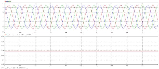
The following diagram shows the window moving over a signal based on the time specified for the window.
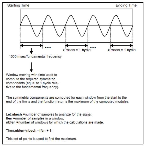
The following figure shows the formulas used to calculate the symmetric components.
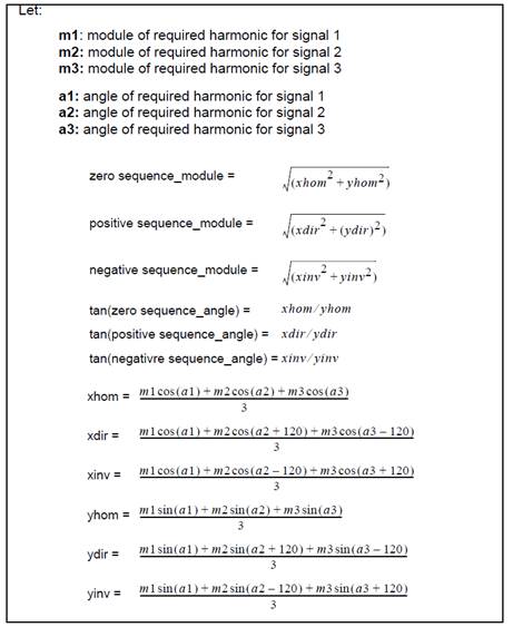
5.8.12. Power and impedance – [sipz]
Compute the power, impedance, addition or subtraction of two signals for a given harmonic.
5.8.12.1. Category
SI5
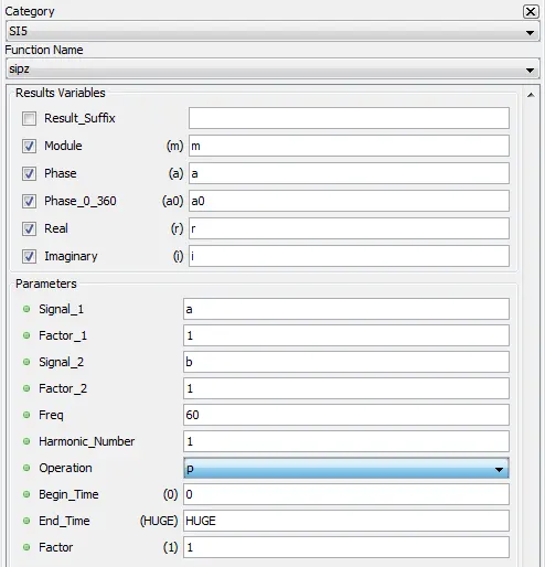
5.8.12.2. Description
This function allows to compute the power, impedance, addition or subtraction of two signals for a given harmonic.
5.8.12.3. Result Variables and Parameters
Module (m): Module (or amplitude) resulting from the operation specified for the harmonic multiplied by the absolute value of the factor.
Phase (a): Angle a (or phase) resulting from the operation specified for the harmonic. Value is between -180 and 180 degrees [°].
Since the module is multiplied by the absolute value of the factor, the phase is modified if the multiplying factor is negative. In this case, 180 degrees are added to the phase.
Phase 0-360 (a0): Angle a0 (or phase) resulting from the operation specified for the harmonic. Value is between 0 and 360 degrees [°].
Real (r): Real part r of the module and angle computed (m * cos(a)).
Imaginary (i): Imaginary part i of the module and angle computed (m * cos(a)).
(m * sin(a)).
Signal_1: First signal to analyze (voltage signal).
Factor_1: Multiplying factor to use for all samples of signal 1.
Signal_2: Second signal to analyze (current signal).
Factor_2: Multiplying factor to use for all samples of signal 2.
Freq: Fundamental frequency of the signals in Hertz [Hz], normally computed with the sifreq function.
Harmonic number: Number of harmonic to compute.
· 0: DC;
· 1: Fundamental;
· 2: 2nd harmonic;
· n: nth harmonic (max. 30).
Operation: Operation to execute on the modules (or amplitudes) and angles of the required harmonic for each input signal. The modules and angles are first computed on the two input signals and then the specified operation is applied to these modules and angles. The defined operators are :
· p : power;
· / : impedance;
· * : multiplication;
· + : addition;
· - : subtraction;
Begin_time: Time at which the analysis of a signal must start. This time is expressed in milliseconds [ms]. This value must be greater than 0 and lower than the duration of the test. The default value is 0.
End_time: Time at which the analysis of a signal must end. This time is expressed in milliseconds [ms]. The value of this time must be larger than the specified begin_time and smaller than the duration of the test. Use the “HUGE” value to specify the end of the test. The default value is HUGE.
The begin_time and end_time specified for the calculation of the harmonics must be the same as those used in the sifreq sequences to compute the fundamental frequency.
Factor: Multiplying factor for the results generated by the function. The default value of the multiplying factor is 1.0 and has no effect on the results.
5.8.12.4. Syntax
[m, a, a0, r, i] = sipz(a, 1, b, 1, 60, 1, "p", 0, HUGE, 1)
5.8.12.5. Characteristics
|
Data type support |
Double Floating point |
5.8.12.6. Example
The first diagram shows how to compute the different powers (p): apparent, active and reactive.
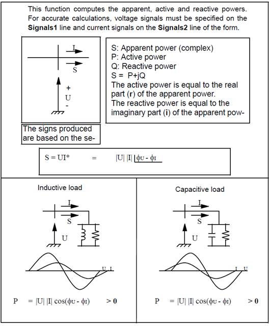
The following diagram shows how to compute the different impedances (/): complex, resistance and reactance.
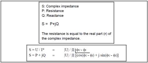
Finally, the next diagram shows the different formulas used with the operations allowed: power (p), impedance (/), addition (+), subtraction (-) and multiplication (*).
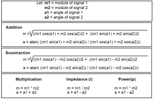
5.8.13. Overshoot Statistics – [siseuil]
Compute overshoot statistics of a signal using a threshold condition.
5.8.13.1. Category
SI5
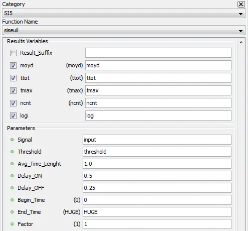
5.8.13.2. Description
This function is used to compute overshoot statistics using a threshold condition. It also generates a logical signal with these overshoot times on the signal studied.
5.8.13.3. Result Variables and Parameters
Moyd: Sample mean computed on the first Time interval (Average Time Length) in milliseconds of the analyzed signal from the start of the signal. Afterwards, the signal overshoots are analyzed from the Starting time.
ttot: Sum of the overshoot times on the threshold value for the signal analyzed. This result is specified in milliseconds [ms].
tmax: Longest overshoot time specified in milliseconds [ms].
ncnt: Number of times when the threshold overshoot duration is longer than the specified Delay ON.
logi: The logical signal has a value of 1 from the start of an overshoot plus the Delay ON value. It remains at 1 until the end of the overshoot plus the specified Delay OFF value. For all other cases, the value of the logical signal is 0. The overshoot times which do not exceed the Delay ON value are not shown in the logical signal.
Threshold (+/-): Difference with the mean of the starting samples to set the threshold value to reach. The threshold value used for overshoot calculations is the threshold difference added to the mean result (the mean of the time interval samples from the start of the study). This difference is expressed in the units of the signals.
Example: Let, the mean moyd = 40.0. If the threshold difference is = 15.0, then the threshold value used is 55.0. If the threshold difference is = -15.0, then the threshold value used is 25.0.
The threshold direction is set by the sign of the threshold. If the difference is negative, then the threshold value is smaller than moyd. Hence, overshoots going towards the bottom part of the graph are looked for, since the start of the study is not considered as an overshoot. This case is shown in first example below. If the difference is positive, then the threshold value is greater than moyd. Hence, overshoots going towards the top part of the graph are looked for, since the start of the study is not considered as an overshoot. This case is shown in the second example.
To be considered as an overshoot, the signal must reach the threshold and return under this threshold within the set limits of the analysis. Thus, if a signal is above a threshold throughout the analysis, then the ncnt, ttot and tmax results will be null.
Average Time Length: Time interval in milliseconds [ms] from time 0 on which the initial mean will be computed and serving to set the threshold. A null value is not valid.
Delay ON: Minimal time during which the overshoot must last in order to be considered as a count. This time is specified in milliseconds [ms].
Delay OFF: Minimal time during which the logical signal generated must stay at 1 following the end of an overshoot. This time is specified in milliseconds [ms].
Begin_time: Time at which the analysis of a signal must start. This time is expressed in milliseconds [ms]. This value must be greater than 0 and lower than the duration of the test. The default value is 0.
End_time: Time at which the analysis of a signal must end. This time is expressed in milliseconds [ms]. The value of this time must be larger than the specified begin_time and smaller than the duration of the test. Use the “HUGE” value to specify the end of the test. The default value is HUGE.
The begin_time and end_time specified for the calculation of the harmonics must be the same as those used in the sifreq sequences to compute the fundamental frequency.
Factor: Multiplying factor for the results generated by the function. The default value of the multiplying factor is 1.0 and has no effect on the results. The factor applies to the moyd, tmax and ttot results.
5.8.13.4. Syntax
[moyd, ttot, tmax, ncnt, logi] = siseuil( input, 0.5, 1.0, 0.5, 0.25, 0, HUGE, 1)
5.8.13.5. Characteristics
|
Data type support |
Double Floating point |
5.8.13.6. Example
The first figure shows a case where the threshold difference is negative.
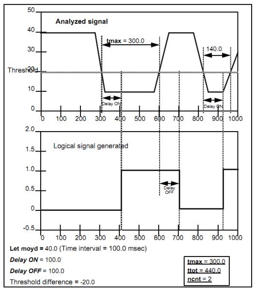
The second figure shows a case where the threshold difference is positive.
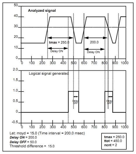
5.8.14. Symmetric components – [sisym3]
Compute the symmetric components of three signals for a given harmonic.
5.8.14.1. Category
SI5
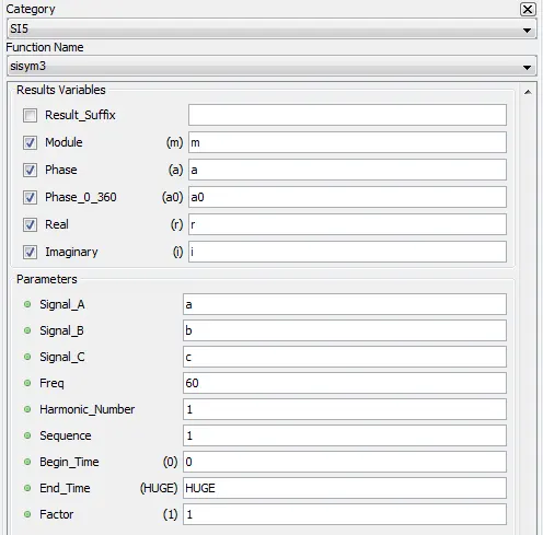
5.8.14.2. Description
This function is used to compute the symmetric components of three signals for a given harmonic. This function computes the module, the phase, and the real and imaginary parts for the symmetric components of a harmonics.
5.8.14.3. Result Variables and Parameters
Module (m): Module (or amplitude) for the symmetric components of a harmonic, multiplied by the absolute value of the factor.
Phase (a): Angle a (or phase) of the symmetric component sequence, between -180 and 180 degrees [°]. Since the module is multiplied by the absolute value of the factor, the phase is modified if the multiplying factor is negative. In this case, 180 degrees are added to the phase.
Phase (a0): Angle of the symmetric component sequence, found between 0 and 360 degrees [°].
Real (r): Real part r of the required symmetric component sequence (m * cos(a)).
Imaginary (i): Imaginary part i of the required symmetric component sequence (m * sin(a)).
Signal_A: First signal to analyze.
Signal_B: Second signal to analyze.
Signal_C: Third signal to analyze.
Freq: Fundamental frequency of the signal in Hertz [Hz], normally computed with the sifreq function.
Harmonic number: Number of harmonic to compute.
· 0: DC;
· 1: Fundamental;
· 2: 2nd harmonic;
· n: nth harmonic (max. 30).
Sequence: Sequence of symmetric components to compute.
· 0: zero sequence
· 1: positive sequence
· 2: negative sequence
Begin_time: Time at which the analysis of a signal must start. This time is expressed in milliseconds [ms]. This value must be greater than 0 and lower than the duration of the test. The default value is 0.
End_time: Time at which the analysis of a signal must end. This time is expressed in milliseconds [ms]. The value of this time must be larger than the specified begin_time and smaller than the duration of the test. Use the “HUGE” value to specify the end of the test. The default value is HUGE.
The begin_time and end_time specified for the calculation of the harmonics must be the same as those used in the sifreq sequences to compute the fundamental frequency.
Factor: Multiplying factor for the results generated by the function. The default value of the multiplying factor is 1.0 and has no effect on the results. The factor applies to the moyd, tmax and ttot results.
5.8.14.4. Syntax
[m, a, a0, r, i] = sisym3( a, b, c, 60, 1, 1, 0, HUGE, 1 )
5.8.14.5. Characteristics
|
Data type support |
Double Floating point |
5.8.14.6. Example
The following diagram shows the mathematical functions used to compute the symmetric components related to three signals.
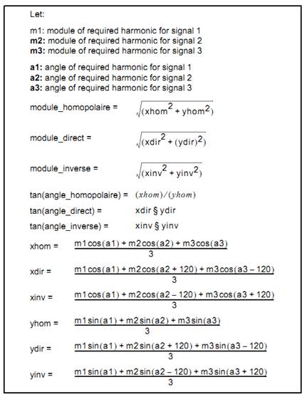
5.8.15. Envelope Overshoot– [sitenv]
Compute the time in milliseconds during which the envelope of a signal overshoots a specific threshold value.
5.8.15.1. Category
SI5
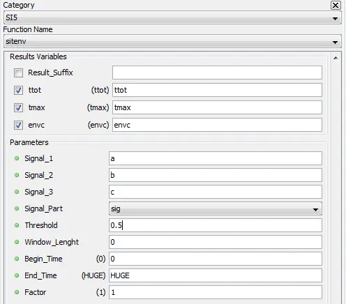
5.8.15.2. Description
This function allows to compute the time in milliseconds [ms] during which the envelope of a signal overshoots a specific threshold value. This function computes the sum, the longest overshoot time and the signal representing the peak envelope.
The peak envelope is a signal consisting of lines connecting the different peaks of a signal. A peak is a sample such that the signals preceding and following it are smaller than the current sample.
5.8.15.3. Result Variables and Parameters
ttot: Sum of the overshoot times for the signal analyzed. This result is specified in milliseconds [ms].
tmax: Longest overshoot time specified in milliseconds [ms].
envc: Signal representing the peak envelope of the absolute maximum envelope for the three initial signals.
Signal_A: First signal to analyze.
Signal_B: Second signal to analyze.
Signal_C: Third signal to analyze.
Signal_Part: Part of the signal on which the analysis is done (neg, pos, sig, abs). Here are the definitions for the four distinct parts of a signal:
- Neg : Only the negative values of the input signal are used for the calculations. The other values are considered to be null.
- Pos : Only the positive values of the input signal are used for the calculations. The other values are considered to be null.
- Sig : The original input signal is used for the calculations.
- Abs : The calculations are done on the absolute value of the input signal.
Threshold: Value of threshold to reach in order to compute the overshoot times. If the threshold is greater than the value of the first sample of the signal analyzed, then the overshoot occurs towards the top part of the signal, and vice versa.
To be considered as an overshoot, the signal must reach the threshold and return under this threshold within the set limits of the analysis. Thus, if a signal is above a threshold throughout the analysis, then the ttot and tmax results will be null.
Window_Length: Time in seconds [s] during which the window moves over the analyzed signal. This time in seconds is reduced to the time of the analysis (end_time – begin_time), if the window time specified is longer than the duration considered for the signal. This window time cannot be null.
Filtering time: Period of mean setting in milliseconds used to filter the envelope signal from the peaks, if required.
Begin_time: Time at which the analysis of a signal must start. This time is expressed in milliseconds [ms]. This value must be greater than 0 and lower than the duration of the test. The default value is 0.
End_time: Time at which the analysis of a signal must end. This time is expressed in milliseconds [ms]. The value of this time must be larger than the specified begin_time and smaller than the duration of the test. Use the “HUGE” value to specify the end of the test. The default value is HUGE.
The begin_time and end_time specified for the calculation of the harmonics must be the same as those used in the sifreq sequences to compute the fundamental frequency.
Factor: Multiplying factor for the results generated by the function. The default value of the multiplying factor is 1.0 and has no effect on the results. The factor can only be applied to the ttot and tmax results.
5.8.15.4. Syntax
[ttot, tmax, envc] = sitenv( a, b, c, "sig", 0.5, 0, 0, HUGE, 1)
5.8.15.5. Characteristics
|
Data type support |
Double Floating point |
5.8.15.6. Example
The following figure, shows the different function calculations for a peak envelope signal.
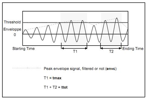
5.8.16. Operating time – [Sitop]
Compute the operating time of a relay.
5.8.16.1. Category
SI5
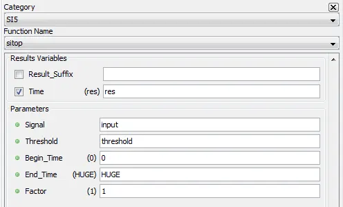
5.8.16.2. Description
This function allows to compute the operating time of a relay.
5.8.16.3. Result Variables and Parameters
Res: time in milliseconds [ms] for which the threshold value is reached on the signal analyzed, as of the specified begin_time. The returned time is the time relative to the starting time and not relative to time 0.
If the returned result is HUGE, this means that the relay did not operate within the set limits. More specifically, no change of state relative to the threshold value was detected within the limits of the analysis, as compared with the state at the beginning of the analysis.
Signal: Signal to analyze.
Threshold: Threshold to reach on the signal analyzed showing that the relay operated. .
The threshold value is reached when there is a change of state with respect to this value. If the sample was above the threshold at the start of the analysis, then the change of state occurs when the sample read is found to be below the threshold value.
Begin_time: Time at which the analysis of a signal must start. This time is expressed in milliseconds [ms]. This value must be greater than 0 and lower than the duration of the test. The default value is 0.
End_time: Time at which the analysis of a signal must end. This time is expressed in milliseconds [ms]. The value of this time must be larger than the specified begin_time and smaller than the duration of the test. Use the “HUGE” value to specify the end of the test. The default value is HUGE.
Factor: Multiplying factor for the results generated by the function. The default value of the multiplying factor is 1.0 and has no effect on the results.
5.8.16.4. Syntax
res = sitop( input, threshold, 0, HUGE, 1)
5.8.16.5. Characteristics
|
Data type support |
Double Floating point |
5.8.16.6. Example
The following figure shows the different cases which can arise when executing the sitop function. These examples can be serve as reference for the cases studied.
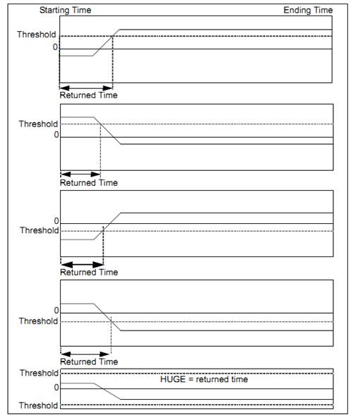
5.8.17. Relative operating time – [sitopref]
Compute the operating time of a relay relative to the rise or fall of a reference signal.
5.8.17.1. Category
SI5
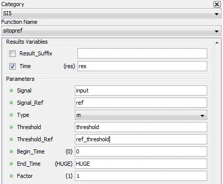
5.8.17.2. Description
The function allows to compute the operating time of a relay relative to the rise or fall of a reference signal.
5.8.17.3. Result Variables and Parameters
res: time in milliseconds for which the threshold value is reached on the signal analyzed, as specified by the reference pulse.
· On a rise (m, c, C), the returned time is relative to the rising time of the reference pulse.
· On a fall (d, f, F), the returned time is relative to the falling time of the reference pulse.
Signal: Signal to analyze.
Reference signal: Reference signal.
Types (m, d, c, C, f, F): Type of search for the relay operating time, in other words the time when a threshold value is reached. On a rise (m, c, C), the relay must operate between the rise of the reference pulse and its end. On a fall (d, f, F), the relay must operate only after the fall of the reference pulse.
· For type m, a change of state is searched for relative to the threshold and the initial state starting time between the start and the end of the reference pulse. If the state is the same at the beginning of the pulse, only a change of state is searched for. If however, the state is different at the beginning of the pulse, the initial state and then a change of state are searched for, both between the start and the end of the reference pulse.
· For type c, a value smaller than the threshold value is searched for, between the start and the end of the reference pulse. If at the beginning of the pulse, the sample is already below the threshold, the search is for a value above the threshold and then for a value below it, before the end of the reference pulse.
· For type C, a value greater than the threshold value is searched for, between the start and the end of the reference pulse. If at the beginning of the pulse, the threshold is already overshot, the search is for a value below the threshold and then for a value above it, before the end of the reference pulse.
· For type f, a value smaller than the threshold value is searched for, between the end of the reference pulse and the ending time. If at the end of the pulse, the sample is already below the threshold, the search is for a value above the threshold and then for a value below it, before the end of the analysis limits.
· For type F, a value greater than the threshold value is searched for, between the end of the reference pulse and the ending time. If, at the end of the pulse, the threshold is already overshot, the search is for a value below the threshold and then for a value above it, before the end of the analysis limits.
Threshold: Threshold to reach on the signal analyzed showing that the relay operated. The method used to establish that the value was reached is determined by the type of search (m, d, c, C, f, F)
Threshold_ref: Threshold value to reach on the reference signal specifying the start and the end of the reference pulse
Begin_time: Time at which the analysis of a signal must start. This time is expressed in milliseconds [ms]. This value must be greater than 0 and lower than the duration of the test. The default value is 0.
End_time: Time at which the analysis of a signal must end. This time is expressed in milliseconds [ms]. The value of this time must be larger than the specified begin_time and smaller than the duration of the test. Use the “HUGE” value to specify the end of the test. The default value is HUGE.
Factor: Multiplying factor for the results generated by the function. The default value of the multiplying factor is 1.0 and has no effect on the results.
5.8.17.4. Syntax
res = sitopref( a, ref, "m", threshold, threshold_ref, 0, HUGE, 1)
5.8.17.5. Characteristics
|
Data type support |
Double Floating point |
5.8.17.6. Example
The following figure shows the different cases for this function, including the limit cases where the values returned are HUGE, -HUGE or simply 0.
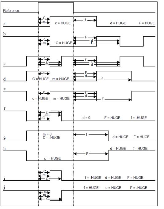
5.8.18. Threshold time – [sitseuil]
Compute the time at which a threshold value is reached.
5.8.18.1. Category
SI5
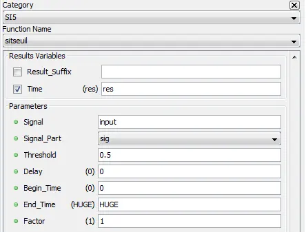
5.8.18.2. Description
Compute the time at which a threshold value is reached (either on positive or negative slope) on a specified part of a signal.
5.8.18.3. Result Variables and Parameters
Result: Time in milliseconds [ms] at which the threshold value is reached on the specified part of the signal, increased by the delay and multiplied by the factor. If the returned result is HUGE, this means that the threshold value was never reached within the set limits
Note that the returned time is really the time at which the threshold value is reached, increased by the delay, and not the time relative to the starting time of the analysis.
Signal: Signal to analyze.
Signal_Part: Part of the signal on which the analysis is done (neg, pos, sig, abs). Here are the definitions for the four distinct parts of a signal:
- Neg : Only the negative values of the input signal are used for the calculations. The other values are considered to be null.
- Pos : Only the positive values of the input signal are used for the calculations. The other values are considered to be null.
- Sig : The original input signal is used for the calculations.
- Abs : The calculations are done on the absolute value of the input signal.
Threshold: Value of threshold to be reached on the specified part of the signal.
Delay: When the threshold time is determined, a delay is added to it. The new starting time of the analysis is thus equal to the time taken to reach the threshold plus the delay. The delay is specified in milliseconds [ms].
Begin_time: Time at which the analysis of a signal must start. This time is expressed in milliseconds [ms]. This value must be greater than 0 and lower than the duration of the test. The default value is 0.
End_time: Time at which the analysis of a signal must end. This time is expressed in milliseconds [ms]. The value of this time must be larger than the specified begin_time and smaller than the duration of the test. Use the “HUGE” value to specify the end of the test. The default value is HUGE.
Factor: Multiplying factor for the results generated by the function. The default value of the multiplying factor is 1.0 and has no effect on the results.
5.8.18.4. Syntax
res = sitseuil( input, "sig", 0.5, 0, 0, HUGE, 1)
5.8.18.5. Characteristics
|
Data type support |
Double Floating point |
5.8.18.6. Example
The following figure shows the different cases which can arise when executing the sitseuil function.
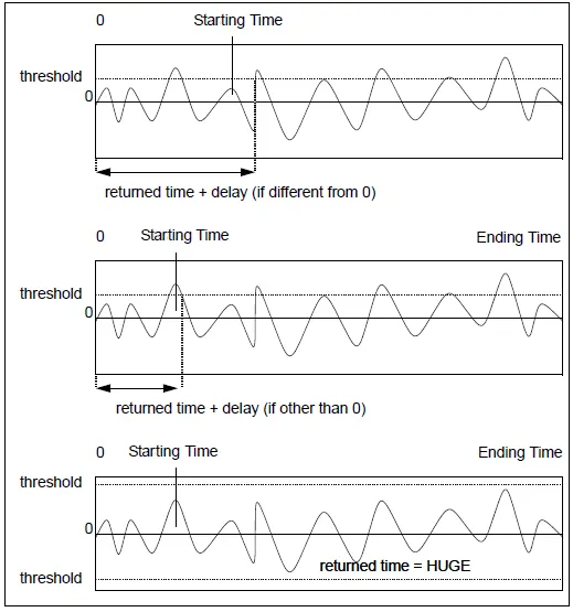
Begin Time: Instant after which the function computes the time.
Pictorial Representation:
![]()
![]()
![]()
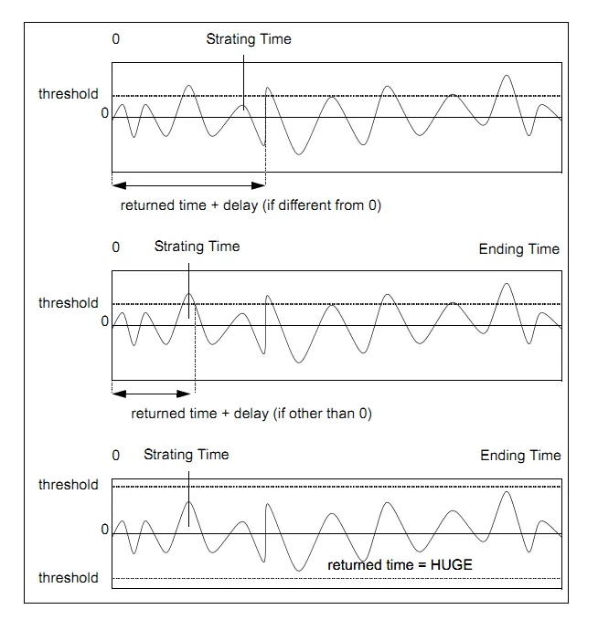
CONTACT
OPAL-RT Corporate Headquarters
1751 Richardson, Suite 2525
Montréal, Québec, Canada
H3K 1G6
Tel.: 514-935-2323
Toll free: 1-877-935-2323
Technical Services
Note:
While every effort has been made to ensure accuracy in this publication, no responsibility can be accepted for errors or omissions. Data may change, as well as legislation, and you are strongly advised to obtain copies of the most recently issued regulations, standards, and guidelines.
This publication is not intended to form the basis of a contract.

28/01/2021
© OPAL-RT TECHNOLOGIES Inc.